
RESEARCH ARTICLE
System Identification of Dampers Using Chaotic Accelerated Particle Swarm Optimization
S. Talatahari1, *, B. Talatahari1, M. Tolouei1
Article Information
Identifiers and Pagination:
Year: 2022Volume: 1
Issue: 1
E-location ID: e200521193450
Publisher ID: e200521193450
DOI: 10.2174/2666782701666210520124649
Article History:
Received Date: 30/11/2020Revision Received Date: 19/03/2021
Acceptance Date: 28/03/2021
Electronic publication date: 24/05/2022

Abstract
Aims: Different chaotic APSO-based algorithms are developed to deal with high non-linear optimization problems. Then, considering the difficulty of the problem, an adaptation of these algorithms is presented to enhance the algorithm.
Background: Particle swarm optimization (PSO) is a population-based stochastic optimization technique suitable for global optimization with no need for direct evaluation of gradients. The method mimics the social behavior of flocks of birds and swarms of insects and satisfies the five axioms of swarm intelligence, namely proximity, quality, diverse response, stability, and adaptability. There are some advantages to using the PSO consisting of easy implementation and a smaller number of parameters to be adjusted; however, it is known that the original PSO had difficulties in controlling the balance between exploration and exploitation. In order to improve this character of the PSO, recently, an improved PSO algorithm, called the accelerated PSO (APSO), was proposed, and preliminary studies show that the APSO can perform superiorly.
Objective: This paper presents several chaos-enhanced accelerated particle swarm optimization methods for high non-linear optimization problems.
Methods: Some modifications to the APSO-based algorithms are performed to enhance their performance. Then, the algorithms are employed to find the optimal parameters of the various types of hysteretic Bouc-Wen models. The problems are solved by the standard PSO, APSO, different CAPSO, and adaptive CAPSO, and the results provide the most useful method. The sub-optimization mechanism is added to these methods to enhance the performance of the algorithm.
Results: Seven different chaotic maps have been investigated to tune the main parameter of the APSO. The main advantage of the CAPSO is that there is a fewer number of parameters compared with other PSO variants. In CAPSO, there is only one parameter to be tuned using chaos theory.
Conclusion: To adapt the new algorithm for susceptible parameter identification algorithm, two series of Bouc-Wen model parameters containing standard and modified Bouc-Wen models are used. Performances are assessed on the basis of the best fitness values and the statistical results of the new approaches from 20 runs with different seeds. Simulation results show that the CAPSO method with Gauss/mouse, Liebovitch, Tent, and Sinusoidal maps performs satisfactorily.
1. INTRODUCTION
System Identification of hysteric non-linear problems determines a set of suitable parameters for a model to match the experimental results with those of the model. In this issue, optimization provides engineers with a variety of techniques to deal with these problems. Due to its highly non-linear nature, identification of Bouc-Wen systems constitutes a challenging problem [1, 2] which has been tackled by a variety ofmethods, such as Gauss-Newton [3], modified Gauss-Newton [4], Least squares [5], Simplex [6], Levenberg–Marquardt [6, 7], extended Kalman filters [6, 8], reduced gradient methods [6], Genetic Algorithms (GAs) [9], real-coded GAs [10], Differential Evolution [11, 12], adaptive laws [13], hybrid evolutionary algorithm [1], Charged System Search (CSS) [2], Particle Swarm Optimization (PSO) [14], a hybrid method based on the PSO and Big Bang-Big Crunch algorithms [15], and many others. These algorithms are known as optimization methods, and some of them [3, 4] are gradient-based methods. Like other classical methods, some issues are present in applying them for system identification problems. Depending on starting point, difficulty in finding gradian information and trapping on local optimums are the most difficult of these algorithms. On the other hand, new meta-heuristic algorithms [1, 2, 9, 10, 14, 15], because of their nature, can be more useful for this problem; however, the performance of these algorithms is not constant, and it differs from one problem to the other one. This shows the requirement of modification on the standard form of these methods to specify them for system identification problems. For example, in one study [2], after adapting the CSS for identification problems, the final results were improved considerably compared to the standard CSS. Considering this point, this paper strives to present some modified, but simple algorithms to solve the identification problems.
Particle Swarm Optimization (PSO) is a population-based stochastic optimization technique suitable for global optimization with no need for direct evaluation of gradients. The method, introduced by Kennedy and Eberhart [16], mimics the social behavior of flocks of birds and swarms of insects and satisfies the five axioms of swarm intelligence, namely proximity, quality, diverse response, stability, and adaptability [17]. The algorithm explores the search space by adjusting the trajectories of individuals, called “particles”, viewed as moving points in the search space. These particles are attracted towards the positions of both their personal best solution and the best solution of the swarm in a stochastic manner [18].
Although there are some advantages to using the PSO consisting of easy implementation and a smaller number of parameters to be adjusted, it is known that the original PSO had difficulties in controlling the balance between exploration and exploitation [19]. In order to improve this character of the PSO, recently, an improved PSO algorithm, called the accelerated PSO (APSO), was proposed, and preliminary studies show that the APSO can perform superiorly, compared with genetic algorithms (GA) and the standard PSO [20]. Later, this method was utilized for optimum design of frame structures by Talatahari et al. [21]. The chaos-enhanced accelerated particle swarm optimization (CAPSO) was proposed by Gandomi et al. [22] in which the important role of randomizing was played by using chaos theory.
Chaotic maps were known as the most efficient tools that could be used instead of random series [23, 24]. Since these maps do not enforce additional computations to the algorithm, as a result, using them can be useful. In this regard, the main contribution of this paper is to present several chaos-enhanced accelerated particle swarm optimization methods for high non-linear optimization problems. Some modifications to these algorithms are performed to enhance their performance. The main idea is based on the Sub-Optimization Mechanism (SOM) [2], in which the search space is divided into several small spaces, and finding optimum solutions becomes easier. Then, the algorithms are employed to find the optimal parameters of the various types of hysteretic Bouc-Wen models. The problems are solved by the standard PSO, APSO, different CAPSO, and adaptive CAPSO, and the results provide the most useful method.
The rest of the paper is organized as follows: Section 2 contains the materials and methods in which the problem definition, utilized methods, and mechanical Bouc-Wen models are presented. Section 3 contains the results and discussion. Section 4 contains the conclusion and policy implications.
2. MATERIALS AND METHODS
2.1. Problem Formulation
The mean square error (MSE) of the predicted response time history
 (for any obtained parameters’ vector p) in comparison with the experimentally obtained response history
 at each time step ti is usually considered as the objective function to be minimized as [2] Eq. (1):
 |
(1) |
in which p is the vector of model’s parameters;
 is the variance of experimental response time history; Σ represents the summation of its subsequent term (N discrete values); and N is the number of experimental data employed in the optimization process. It should be noted that the optimization problem involves the minimization of the objective function when the parameters vector is varied between the following side constraints, see Eq. (2):
 |
(2) |
where pmin and pmax are the vectors that include the lower and upper bounds of the model parameters, respectively.
2.2. Standard Particle Swarm Optimization (PSO)
The PSO algorithm, inspired by social behavior simulation [16], is a population-based optimization algorithm that involves a number of particles that move through the search space, and their positions are updated based on the best positions of individual particles (called
 ) and the best of the swarm (called
 ) in each iteration. This matter is shown mathematically as the following equations (3, 4)):
 |
(3) |
 |
(4) |
where xi and vi represent the current position and the velocity of the ith particle, respectively. rand1 and rand2 represent random numbers between 0 and 1; is the best position visited by each particle itself;
corresponds to the global best position in the swarm up to iteration
 represent cognitive and social parameters, respectively. According to Kennedy and Eberhart [16], these two constants are set to 2 in order to make the average velocity change coefficient close to one. \is a weighting factor (inertia weight) that controls the trade-off between global exploration and local exploitation abilities of the flying particles. A larger inertia weight makes global exploration easier, while a smaller inertia weight tends to facilitate local exploitation. The inertia weight can be reduced linearly from 0.9 to 0.4 during the optimization process [25].
2.3. Accelerated Particle Swarm Optimization
The standard PSO uses both the current global best
and the individual best,
. The reason for using the individual best is primarily to increase the diversity in the quality solutions. However, this diversity can be simulated using some randomness. Subsequently, there is no compelling reason for using the individual best unless the optimization problem of interest is highly non-linear and multimodal [20].
A simplified version that could accelerate the convergence of the algorithm uses the global best only. Thus, in the Accelerated Particle Swarm Optimization (APSO) [20], the velocity vector is generated by a simpler formula as Eq. (5):
 |
(5) |
where randn is drawn from N(0, 1) to replace the second term. The update of the position is simply like Eq. (4). In order to increase the convergence even further, we can also write the update of the location in a single step, as Eq. (6)
 |
(6) |
This simpler version will give the same order of convergence [1]. Typically, α = 0.1L -0.5L, where L is the largest of the search space for each variable, while β = 0.2 -0.7 is sufficient for most applications. It is worth pointing out that the velocity does not appear in Eq. (6), and there is no need to deal with the initialization of velocity vectors. Therefore, the APSO is much simpler. Comparing with many PSO variants, the APSO uses only two parameters, and the mechanism is simple to understand. A further improvement to the accelerated PSO is to reduce the randomness as iterations proceed. In our implementation, we use Eq. (7) [22]
 |
(7) |
where tϵ[0, tmax] and tmax is the maximum number of iterations.
2.4. Chaotic APSO
As it is presented in Eq. (6), the main parameter of the APSO is the learning parameter, β. The parameter β characterizes the variations of the global best attraction, and its value is crucially important in determining the speed of the convergence and the behavior of APSO. Based on a parametric study, by varying b from 0 to 1 by a step of 0.1, we found that b should be in [0.2, 0.7] for most problems [22]. In the standard APSO, there is no need to keep β constant. In fact, a varying β may be advantageous, which may also lead to the speedup of convergence of the algorithm. As all chaotic maps are normalized, the variations of a chaotic map are always between [0, 1]. Therefore, chaotic maps can be used to tune parameter β, and such chaotic-enhanced APSO is referred to as the chaotic APSO (CAPSO). Different chaotic maps are utilized for CAPSO, as summarized in Table 1.
For presenting more efficient algorithms, the Sub-Optimization Mechanism (SOM) [2] is added to the CAPSO methods. This mechanism is based on the principles of the finite element method that requires division of the problem domain into many sub-domains, and each domain is called a finite element. These element patches are considered instead of the main domain. Similarly, SOM divides the search space into sub-domains and performs an optimization process into these patches, and then based on the resulting solutions, the undesirable parts are deleted. The remaining space is divided into smaller parts for more investigation in the next stage. This process continues for determining numbers or until the remaining space gets less than the required accuracy or specified value [2].
| Name | Equation | Condition |
|---|---|---|
| Gauss/mouse map |

|

|
| Circle map |

|
a = 0.5 and b = 0.2 |
| Logistic map |

|

|
| Sinusoidal map |

|
|
| Tent map |

|
- |
| Liebovtech map |

|
|
| Sinus map |

|
- |
For parameter identification of the Bouc-Wen model for MR dampers, the adaptive CAPSO method utilizes the idea of the SOM as the following steps:
Level 1: Employing the standard algorithm considering the defined search domain to find the optimum results. In this step, the search process can be circumscribed to only 100 iterations.
Level 2: Determining a new search domain for each variable using the optimum results obtained in the previous level. Using the information obtained in the previous search (Xopt), it is possible that the search domain becomes defined again more accurately. In this way, the previous optimum result is considered as the center point of the domain, and the domain will be as Eq. (8):
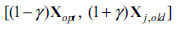 |
(8) |
where γ is the domain limit and is set to 0.1 for the next repetitions.
Level 3: Repeating above levels for definite times (three times in this paper).
Fig. (1) presents a simple flow-chart of using CAPSO for the defined problem.
2.5. Mechanical Bouc-Wen Models for MR Dampers
The standard Bouc-Wen model [26] and a modified one were considered in this paper to be capable of reproducing the factual non-linear hysteretic behavior of MR dampers.
2.5.1. Standard Bouc-Wen Model
Fig. (2a) illustrates the simple Bouc-Wen model for MR dampers. In this case, the non-linear force of the damper is calculated from Eq. (1) as follows Eq. (9) [26]:
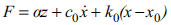 |
(9) |
where, α is the Bouc-Wen model parameter related to the MR material yield stress; k0 and c0 are spring stiffness and dashpot damping coefficient, respectively; and z is hysteretic deformation of the model which is defined by the following equation (9):
 |
(10) |
in which, A, β and γ are the Bouc-Wen model parameters.
For achieving optimal performance of control systems equipped with MR dampers, the applied voltage to the current driver must be varied according to the measured feedback at any moment to change the damping force. Thus, for accounting this accordance, the coefficient α, damping coefficient c0, and stiffness k0 in Eq. (9) are defined as a linear function of the efficient voltage as given by the following equations (11, 12)) [27]:
 |
(11) |
To accommodate the dynamics involved in the MR fluid reaching rheological equilibrium, the following first-order filter is employed to calculate efficient voltage, u by Eq. (12) [27]:
 |
(12) |
where v is the applied voltage for the current generation.
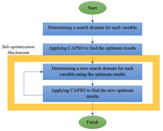 |
Fig. (1). Flow-chart of applying the CAPSO algorithm. |
 |
Fig. (2). The phenomenological Bouc-Wen model of MR damper schematic a) simple, b) modified. |
2.5.2. Modified Bouc-Wen Model
A modified version has been proposed to better predict the roll-off in MR damper force for the region with low velocities. This system is illustrated in Fig. (2b), and generated force by MR damper is given by Eq. (13).
 |
(13) |
In this case, hysteretic displacement z is given by Eq. (14)
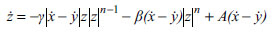 |
(14) |
According to (Fig. 2b),
 is defined by the following equation (15):
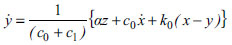 |
(15) |
To determine a comprehensive model that is valid for fluctuating magnetic fields, the parameters α, c0 and c1 in Eqs. (13) and (15) are defined as a linear function of the efficient voltage, u, as given by Eq. (8), see Eq. (16) [27]:
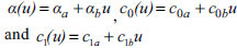 |
(16) |
in which u is related to applied voltage through Eq. (12).
3. Results and Discussion
The standard Bouc-Wen model needs twelve parameters
 while 14 ones
 are sufficient for the modified version.
Two numerical examples for the standard and modified Bouc-Wen models of dampers are optimized utilizing the proposed APSO method. Table 2 presents the used experimental data [2]. The sample displacement and control voltage history are applied simultaneously to the MR damper, and the assumed experimental results for the standard model are shown in Fig. (3) [27]. To fulfill this aim, a series of realistic Bouc-Wen model parameters for a prototype 1000kN MR damper is used to numerically generate the experimental data. It has been corroborated that the simple Bouc-Wen model suffers from parameter redundancy, and multiple sets of parameters could be the solution of a specified problem resulting in similar fairly low MSE.
The device is assumed to be in a real operating condition that an MR damper will experience while it is employed in a semi-active control system of a building. In other words, to accurately evaluate the performance of the identification algorithm, experimental data are obtained due to just one representative test of random inputs (displacement and voltage) to the damper. The input control signal, piston movement, and response of the MR damper for the simple Bouc-Wen model is determined from numerical simulation of a 3-storey case-study building in which a direct modulating controller was designed in order to control the dampers’ force and mitigation of structural responses due to El Centro Earthquake, and for the modified model it is determined from numerical simulation of a 11-storey example subjected to El Centro earthquake controlled using clipped-optimal control algorithm. The sample displacement and control voltage history are applied simultaneously to the MR damper.
The statistical results using 7 variants of the presented algorithms, 7 adaptive methods, the standard PSO, and the APSO are summarized in table 3 and 4 for the standard and modified Bouc-Wen models, respectively. Each algorithm is utilized 20 times with different initial seeds. For the standard model, many of the adaptive chaotic-based APSO methods can find suitable results successfully. However, the best solutions found by Gauss/mouse, Sinusoidal, Liebovitch, and Tent map are better than the best solutions found by the other techniques. Also, it can be seen that the average searching quality of the adaptive CAPSO algorithm with Gauss/mouse and Tent maps is better than those of other methods. In the modified model, the best results are obtained by the adaptive CAPSO methods with Gauss/mouse, Liebovitch, Tent and Sinusoidal maps, respectively. The adaptive CAPSO with Gauss/mouse map has the best performance regarding the standard deviation.
Table 5 presents the best obtained results of the adaptive CAPSO methods for the simple model. From the table, it comes that many of chaotic-based developed algorithms could find a good estimation of optimal solutions for the parameters of standard Bouc-Wen model. The achieved results for modified Bouc-Wen model reported in Table 6 similarly reveal that the proposed optimization methods outperform the original and improved PSO algorithms.
| Parameter | Unit |
Stanard B-W Model Values (9 Parameters) |
Modified B-W Model Values (13 Parameters) |
|---|---|---|---|
| x0 | m | - | - |
| γ | m-2 | 141 | 164 |
| β | m-2 | 141 | 164 |
| A | - | 2075 | 1107.2 |
| n | - | 2 | 2 |

|
kN/m | 26 | 46.2 |

|
kN/m/V | 29.1 | 41.2 |
| c0a | kN.s/m | 105.4 | 110 |
| c0b | kN.s/m/V | 131.6 | 114.3 |
| c1a | kN.s/m | - | 8359.2 |
| c1b | kN.s/m/V | - | 7482.9 |
| k0 | kN/m | - | 0.002 |
| k1 | kN/m | - | 0.0097 |
| η | s-1 | 100 | 100 |
 |
Fig. (3). Numerically obtained experimental data for the standard Bouc-Wen model of a 1000 kN MR damper under the control system simulation [25], a) Force-Time, b) Force-Velocity, c) Voltage-Time. |
| - | Best | Mean | Worst | Std. Dev. |
|---|---|---|---|---|
| Standard PSO, [15] | 5.15E-02 | 1.39 E -01 | 2.73 E -01 | 8.12 E -02 |
| ICA, [27] | 6.28E-03 | 1.26 E -01 | 7.01 E -01 | 3.36 E -01 |
| EICA, [27] | 9.16E-04 | 9.08 E -02 | 2.36 E -01 | 9.66 E -02 |
| APSO | 2.67 E -03 | 8.65 E -02 | 2.25 E -01 | 7.52 E -02 |
| CAPSO with | - | - | - | - |
| Gauss/mouse map | 2.99 E -04 | 7.48 E -02 | 3.26 E -01 | 1.10 E -01 |
| Circle map | 9.49 E -03 | 1.43 E 00 | 17.91 E 00 | 1.27 E 00 |
| Logistic map | 3.78 E -03 | 1.27 E 00 | 3.51 E 00 | 1.45 E 00 |
| Sinusoidal map | 3.09 E -04 | 1.11 E -01 | 5.66 E -01 | 1.19 E -01 |
| Tent map | 5.91 E -04 | 7.85 E -02 | 4.44 E -01 | 1.90 E -01 |
| Liebovitch map | 3.59 E -04 | 4.25 E -02 | 5.21 E -01 | 1.06 E -01 |
| Sine map | 7.77 E -04 | 9.73 E -02 | 8.12 E -01 | 4.63 E -01 |
| Adaptive-CAPSO with | - | - | - | - |
| Gauss/mouse map | 1.200 E -04 | 4.104 E -2 | 1.85E-01 | 6.36 E -02 |
| Circle map | 8.103 E -03 | 8.442 E -1 | 9.98 E 00 | 9.97 E -01 |
| Logistic map | 1.634 E -03 | 9.680 E -1 | 2.96 E 00 | 8.65 E -01 |
| Sinusoidal map | 2.024 E -04 | 8.610E-2 | 2.46 E -01 | 7.22 E -02 |
| Tent map | 3.839 E -04 | 5.660E-2 | 1.69 E -01 | 6.85 E -02 |
| Liebovitch map | 2.478 E -04 | 2.049E-2 | 2.56 E -01 | 9.52 E -02 |
| Sine map | 5.255 E -04 | 7.045 E-2 | 5.28 E -01 | 3.09 E -01 |
| - | Best | Mean | Worst | Std. Dev. | ||||
|---|---|---|---|---|---|---|---|---|
| Standard PSO, [15] | 1.08E-2 | 6.70 E -1 | 1.69 E 00 | 6.93 E -01 | ||||
| ICA, [27] | 1.05 E -02 | 5.68 E -01 | 1.03 E 00 | 5.65 E -01 | ||||
| CICA, [27] | 7.78 E -04 | 3.69 E -01 | 9.65 E -01 | 2.23 E -01 | ||||
| APSO | 2.658 E -3 | 5.35 E -01 | 8.89 E -01 | 5.68 E -01 | ||||
| CAPSO with | - | - | - | - | ||||
| Gauss/mouse map | 7.55 E -04 | 1.482 E -01 | 1.27 E 00 | 8.73 E -02 | ||||
| Circle map | 8.44 E -03 | 2.19 E 00 | 2.23 E 00 | 1.46 E 00 | ||||
| Logistic map | 2.03 E -03 | 2.08 E 00 | 1.21 E +01 | 1.75 E 00 | ||||
| Sinusoidal map | 5.909 E -03 | 6.83 E -01 | 1.06 E 00 | 0.101 E -01 | ||||
| Tent map | 1.152 E -03 | 5.22 E -01 | 1.35 E +01 | 0.167 E -01 | ||||
| Liebovitch map | 6.13 E -04 | 5.13 E -01 | 9.17 E -01 | 0.141 E -01 | ||||
| Sine map | 4.599 E -3 | 1.12 E 00 | 1.18 E 00 | 0.996 E -01 | ||||
| Adaptive-CAPSO with | - | - | - | - | ||||
| Gauss/mouse map | 3.343 E-4 | 8.72 E -2 | 6.93 E -1 | 6.981 E -02 | ||||
| Circle map | 6.299 E -3 | 1.163 E +0 | 1.781 E 0 | 9.067 E -01 | ||||
| Logistic map | 1.032 E -3 | 1.065 E +0 | 6.689 E 0 | 1.188 E +00 | ||||
| Sinusoidal map | 4.421 E -3 | 4.415 E -1 | 8.59 E -1 | 7.459 E -02 | ||||
| Tent map | 6.583 E-4 | 4.594 E -1 | 7.00 E 0 | 9.168 E -02 | ||||
| Liebovitch map | 4.088 E -4 | 4.472 E -1 | 6.80 E-1 | 8.932 E -02 | ||||
| Sine map | 2.389 E -3 | 8.968 E -1 | 9.88 E -1 | 6.431 E -01 | ||||
| Parameter | Unit | CAPSO with | ||||||
|---|---|---|---|---|---|---|---|---|
| - | - | Gauss/mouse | Circle | Logistic | Sinusoidal | Tent | Liebovitch | Sine |
| γ | m-2 | 154.76 | 151.29 | 141.98 | 163.46 | 155.51 | 158.89 | 158.50 |
| β | m-2 | 142.59 | 142.59 | 142.22 | 141.28 | 148.44 | 145.7 | 150.58 |
| A | - | 2058.3 | 2145.0 | 1947.7 | 2100.9 | 2101.8 | 1945.5 | 2103.3 |
| n | - | 1.99 | 2.02 | 1.93 | 1.92 | 1.99 | 1.90 | 1.97 |
|
|
kN/m | 27.97 | 25.68 | 27.09 | 27.20 | 26.27 | 27.32 | 25.45 |
|
|
kN/m/V | 29.61 | 28.54 | 30.87 | 29.15 | 29.38 | 29.63 | 29.16 |
| c0a | kN.s/m | 99.96 | 94.76 | 92.00 | 102.18 | 105.81 | 96.61 | 97.61 |
| c0b | kN.s/m/V | 131.26 | 131.10 | 131.15 | 131.23 | 131.21 | 131.13 | 131.08 |
| η | s-1 | 100.28 | 100.52 | 99.70 | 100.23 | 100.20 | 100.06 | 98.88 |
| - | - | Adaptive CAPSO with | ||||||
|---|---|---|---|---|---|---|---|---|
| Parameter | Unit | Gauss/mouse | Circle | Logistic | Sinusoidal | Tent | Liebovitch | Sine |
| γ | m-2 | 162.27 | 153.78 | 160.81 | 154.62 | 154.98 | 156.94 | 157.48 |
| β | m-2 | 162.26 | 160.08 | 158.59 | 154.4 | 168.87 | 159.32 | 165.45 |
| A | - | 1152.61 | 1126.91 | 1132.42 | 1244.605 | 1180.774 | 1127.862 | 1090.616 |
| n | - | 2.01 | 1.98 | 2.06 | 2.03 | 1.95 | 1.91 | 2.00 |
|
|
kN/m | 45.44 | 45.91 | 45.01 | 45.59 | 46.66 | 44.88 | 46.56 |
|
|
kN/m/V | 40.54 | 35.92 | 42.11 | 40.19 | 39.87 | 36.87 | 38.98 |
| c0a | kN.s/m | 112.62 | 106.13 | 109.03 | 105.71 | 111.08 | 112.3 | 101.33 |
| c0b | kN.s/m/V | 113.96 | 114.67 | 113.71 | 113.01 | 114.66 | 114.11 | 112.68 |
| c1a | kN.s/m | 8035.5 | 8345.5 | 8213.9 | 8315.3 | 8247.2 | 8474.4 | 8429.8 |
| c1b | kN.s/m/V | 7548.8 | 7536.1 | 7451.3 | 7386.6 | 7464.3 | 7472.3 | 7403.8 |
| k0 | kN/m | 0.0021 | 0.0019 | 0.002 | 0.0019 | 0.0021 | 0.0018 | 0.002 |
| k1 | kN/m | 0.0087 | 0.0095 | 0.0094 | 0.0097 | 0.0099 | 0.0099 | 0.0101 |
| η | s-1 | 100.24 | 100.19 | 101.08 | 100.23 | 101.32 | 101.21 | 100.12 |
| Main Algorithm | Example | Data Type | Alternative Algorithms | |||
|---|---|---|---|---|---|---|
| PSO | APSO | ICA | EICA | |||
| CAPSO | Simple B-W model | Min. | 1.258E-17 | 7.15E-12 | 6.17E-05 | 2.95E-04 |
| Mean | 5.32E-14 | 2.22E-11 | 4.49E-06 | 4.78E-04 | ||
| Std. | 5.66E-12 | 3.17E-9 | 6.55E-04 | 8.25E-03 | ||
| Modified B-W Model |
Min. | 7.74E-10 | 7.63E-05 | 6.99E-04 | 1.67E-02 | |
| Mean | 2.35E-09 | 9.34E-04 | 3.59E-05 | 3.59E-03 | ||
| Std. | 3.45E-08 | 6.90E-03 | 9.32E-03 | 3.10E-02 | ||
| Rankings | Min. | Mean | Std. | |||
|---|---|---|---|---|---|---|
| Algorithms | Mean of Ranks | Algorithms | Mean of Ranks | Algorithms | Mean of Ranks | |
| 1 | CAPSO | 320.23 | CAPSO | 312.12 | CAPSO | 300.52 |
| 2 | EICA | 360.11 | EICA | 333.22 | APSO | 315.22 |
| 3 | APSO | 362.22 | APSO | 352.36 | EICA | 316.52 |
| 4 | ICA | 378.56 | ICA | 380.25 | PSO | 370.23 |
| 5 | PSO | 400.52 | PSO | 445.23 | ICA | 460.44 |
| Chi-sq. | 153.15 | 140.52 | 183.35 | |||
| Prob>Chi-sq. | 5.32E-28 | 3.25E-23 | 5.12E-33 | |||
Also, to evaluate the performance of the presented algorithm, a statistical analysis has been conducted in which the Wilcoxon signed-rank (W) test is conducted for comparing the mean ranks of different metaheuristics and the Kruskal–Wallis (K-W) test is conducted for comparing the overall rankings of the metaheuristics by considering the mean of the ranks of algorithms. The Wilcoxon (W) singed-rank test is a statistical nonparametric test for examining the differences between different samples in a one-by-one manner. The related p-values of this test for different methods are presented in Table 7. The Kruskal-Wallis (K-W) test is a non-parametric algorithm for testing whether or not different statistical samples are originated from the same distribution. It is used for comparing two or more independent samples of equal or different sample sizes. This test provides the mean of the ranks for multiple sets of statistical data which are considered for comparing analysis. The results of the K-W test are presented in Table 8. Based on the statistical results, the superiority of the new algorithm is proved.
SUMMARY AND CONCLUSION
A new identification method for non-linear hysteretic Bouc-Wen models of MR fluid dampers is introduced by the different Chaotic Accelerated Particle Swarm Optimization methods as the main contribution of the paper. Seven different chaotic maps have been investigated to tune the main parameter of the APSO. The main advantage of the CAPSO is that there are a fewer number of parameters, compared with other PSO variants. In CAPSO, there is only one parameter to be tuned using chaos theory. Also, the sub-optimization mechanism is added to these methods to enhance the performance of the algorithm.
To adapt the new algorithm for susceptible parameter identification algorithm, two series of Bouc-Wen model parameters containing standard and modified Bouc-Wen models are used. Performances are assessed on the basis of the best fitness values and the statistical results of the new approaches from 20 runs with different seeds. Simulation results show that the CAPSO method with Gauss/mouse, Liebovitch, Tent, and Sinusoidal maps performs satisfactorily.
CONSENT FOR PUBLICATION
Not applicable.
AVAILABILITY OF DATA AND MATERIALS
The authors confirm that the data supporting the results and findings of this study are available within the article.
FUNDING
This research was financially supported by the University of Tabriz (Grant No.1615), Iran.
CONFLICT OF INTEREST
The authors declare no conflict of interest, financial or otherwise.
ACKNOWLEDGEMENTS
The authors of the present survey would like to thank all the participants who enrolled in this study.