
RESEARCH ARTICLE
Application of Support Vector Regression and Time Series Method in Short-term Power Load Forecasting with Regional Difference
Li-Ling Peng1, Song-Qiao Dong1, Meng Yu1, Guo-Feng Fan1, *, Wei-Chiang Hong2
Article Information
Identifiers and Pagination:
Year: 2021Volume: 1
Issue: 1
E-location ID: e190721194078
Publisher ID: e190721194078
DOI: 10.2174/2666782701666210614223415
Article History:
Received Date: 23/03/2021Revision Received Date: 22/05/2021
Acceptance Date: 26/05/2021
Electronic publication date: 14/06/2021

Abstract
Aim: The aim of this study is to perform short-term load forecasting.
Background: Short-term load forecasting plays a key role in power dispatching. It provides basic data for basic power generation planning and system safety analysis so that the power dispatching work is more practical and the power generation efficiency is higher.
Objective: The aim of this study is to ensure the safe operation of the electricity market and relieve the pressure of supply and demand.
Methods: In this paper, the SVR model is used for short-term load prediction.
Results: The SVR model has the advantage of minimizing the structural risk and has good generalization performance for the predicted object. At the same time, the global optimization is ensured, a lot of mapping calculation is reduced, the actual risk is reduced, and the prediction performance is improved.
Conclusion: The target model has higher forecasting accuracy than other forecasting models and can effectively solve the problems of the power market.
1. INTRODUCTION
In recent years, due to the establishment and development of domestic and foreign power markets, the prediction of power load has gradually become the main module of the economization of power system operation and the construction of smart grid [1], and it is also an important research topic in the field of power. Accurate load forecasting can arrange the start-up and shut-down of generator sets and the maintenance plan of power transmission and transformation equipment in the power system so as to meet the social needs, reduce unnecessary energy waste and reduce costs. It would improve economic and social performance. Especially in the case of power management marketization, power load forecasting is particularly important. Through accurate load prediction and precise demand response, strategies can be developed to reduce peak loads and electricity consumption, and integrate distributed energy resources [2, 3]. Therefore, it has brought significant economic benefits to the local economy [4]. In today's power big data environment, aiming at the complexity and uncertainty of power systems [5], there are also many research works on power load forecasting in the market. At present, common traditional models include artificial neural networks, empirical mode decomposition, grey theory [6], multiple linear regression, time series [7], random forest, and decision tree. However, the prediction accuracy and real-time demand of these methods cannot meet the need of the economic market because of the fuzziness and non-linearity of power load. According to the complexity of power load, Mohamed et al. [8] proposed a probabilistic deep convolutional neural network method, which can predict load in the form of quantiles. Case studies have shown that this method has good performance. Ma et al. [9] proposed an interval prediction method based on optimized machine learning and neural network, which not only simplified the prediction process and shortened the processing time, but also significantly improved the efficiency, flexibility, and accuracy of the prediction. Fan et al. [10] proposed a multiple target depth based on the empirical mode decomposition belief network prediction method (EMD - MODBN); the test results have shown that this method has obvious advantages in predicting accuracy and generalization ability. Qiu et al. [11] proposed a short-term power load forecasting method with correction error by dynamic modal decomposition, which has the advantage of good stability. However, the above-mentioned methods have limitations and greater risks, and the mapping calculation is more complex [12-14]. The Time Series model proposes a combination method of short-term load prediction based on fuzzy time series and convolutional neural network to determine and extract relevant important parameters. Various experiments on test data sets proved the effectiveness of this method, but the steps were relatively complex. Grzegorz et al. [15] proposed a univariate short-term power load prediction model based on linear regression and compared this method with ARIMA, exponential smoothing, and neural network models and found that it had a good prediction effect. Wu et al. [16] proposed a new short-term power load forecasting method based on the LRD-regression comprehensive moving average FARIMA model and tested different forecasting models. The results showed that the FARIMA model and the improved optimization algorithm have high accuracy and effectiveness for short-term power load prediction. Gopal et al. [17] proposed a robust framework for short-term power load prediction with test cases involving five commercial buildings with five different building types. The load prediction results showed that the deep learning algorithm RNN improved the performance of load prediction. Shahzad et al. [18] proposed a prediction method based on LSTM, which has the potential to further improve the prediction accuracy. Ahmad et al. [19] proposed a random forest power load prediction method, which calculated the optimal parameters of the support vector machine based on the least square method. Finally, an example showed that the method has fast operation speed and high prediction accuracy. Guo et al. [20] discussed three commonly used machine learning methods for load prediction, namely support vector machine method, random forest regression method, and short-term memory neural network method. Combined with the advantages of these methods, a fusion prediction method and data processing technology were proposed to improve the prediction accuracy.
To sum up, power short-term load data has the characteristics of transient, non-stationary, and randomness. In this paper, the SVR model was used for short-term load forecasting and compared with the ARIMA model after EMD. The main research contents are as follows: (1) Firstly, the data were divided into the training set and validation set, and then the advantages of linear separability and structural risk minimization of support vector machine were used as the basis of training set prediction. (2) The EMD method was used to decompose the original power load data to generate IMF, which was divided into three components according to its characteristics of high, medium, and low frequency. Then, it was combined into two parts (M1 and M2) for prediction by the time series method, and the predicted values were obtained, respectively. (3) Then, the prediction error was calculated for the original value and the predicted value, and the model with higher prediction accuracy was selected by comparing the evaluation indexes. By comparing the prediction effects of SVR and EMD-ARIMA in different regions, this paper explains which model is more suitable for revealing the mechanism of power behavior. The second part introduces the support vector machine regression SVR model, EMD method, and ARIMA in the time series model in detail. The third part takes the power load data of three regions (CAPITL, CENTRL and DUNWOD) as an example to establish the corresponding model for short-term load prediction and analysis. The fourth part compares the predicted results of the model and then draws the corresponding comparison chart between the predicted value and the actual value for analysis. Finally, the regional differences of the three cities (CAPITL, CENTRL and DUNWOD) are compared. The fifth part briefly summarizes the research results of this paper.
2. MATERIALS AND METHODS
2.1. Support Vector Regression Model
Support Vector Machine (SVM) is a set of learning algorithms proposed at the end of the 20th century, which can efficiently solve practical problems such as small samples, non-linearity, and high dimensions [21]. From an ideological point of view, SVM simplifies common issues such as classification and regression. A few support vectors determine the final decision function of SVM, and the complexity of calculation depends on the support vectors rather than the whole sample space, thus avoiding the “dimension disaster”.
The specific steps of the SVR model are as follows:
1. Given the training sample set:
 where
where
 is the input vector (including factors affecting the output),
 is the target output and is the number of samples contained in the sample set. In real life, we often have nonlinear problems; therefore, we need to use mapping function
 to map the sample points to a high-dimensional space
 .
.
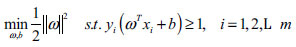
2. In the sample space, the partitioning hyperplane can be described by the following linear Equation (1):
 |
(1) |
 is the normal vector, which determines the direction of the hyper-plane; and b is the displacement term, which determines the distance between the hyper-plane and the origin.
3. Assuming that the hyper-plane
 can classify the training samples correctly, that is for
 if
if
 (Equation 2). Therefore,
 |
(2) |
4. Fig. (1) shows that the distance between the two dotted lines in the SVR soft segmentation hyper-plane is
 which is called the interval. If a partition hyper-plane with “maximum margin” is found, such as parameters
 and b, it makes
 maximum given as:
 |
(3) |
The above constraint (Equation 3) is equivalent to the following constraint (Equation 4):
 |
(4) |
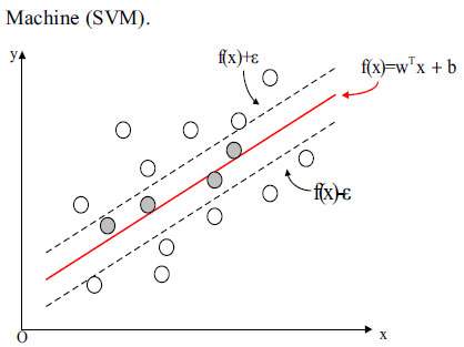 |
Fig. (1). SVR soft segmentation hyper-plane. |
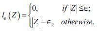
The SVR can be represented by Equation (5):
 |
(5) |
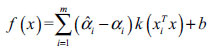
Where C is the regularization constant and
 (Equation 6) is the insensitive loss function of
 as shown in the Figure (1):
 |
(6) |
By introducing the relaxation variables, ξi and (ξi) SVR can be expressed as follows in Equation (7):
 |
(7) |
The corresponding SVR modeling flow chart is shown in Fig. (2).
2.2. EMD
Empirical Mode Decomposition (Empirical Mode Decomposition, the EMD) method is based on the time scale characteristics of the data itself for signal decomposition. It does not need to set any basis function in advance to process non-stationary and nonlinear data. It is suitable for analyzing nonlinear and non-stationary signal sequences and has a high signal-to-noise ratio. The EMD decomposition process is as follows:
I. Finding all the extreme points of the original data sequence X(t), calculating the upper and lower envelopes and denoting its mean value as ml. By using h1 = X(t)-ml. A new low-frequency data sequence h1 is obtained.
II. Repeating the above process so that the first eigenmode function component c1, which represents the highest frequency component of the signal data sequence, can be obtained.
III. Subtracting c1 from X(t), which gives a new data sequence R1, and removing the high-frequency components that are decomposed. This is repeated until the data sequence cannot be decomposed, and this sequence is the mean of X(t).
 |
Fig. (2). Flow chart of SVR modeling. |
2.3. Model Establishment
In this paper, the load series data of three regions are studied, and the predicted values obtained by the correlation prediction method are used for correlation analysis to reflect the regional differences. The steps are as follows:
1. The data is divided into a training set and a validation set. The advantages of linear separability of support vector machine and structural risk minimization are used as the basis of training set prediction, and the predicted value Y1 is obtained.
2. The EMD method is used to decompose the original power load data to generate IMF, which is divided into three components. According to its characteristics, it is divided into three components high, medium and low frequency.
3. Then, the prediction error is calculated for the original value and the predicted value, and the model with higher prediction accuracy is selected by comparing the evaluation indexes.
Fig. (3) presents the flow chart of the short-term load forecast based on the SVR model, clearly showing the above steps.
3. NUMERICAL STUDY
3.1. Data Sets and Evaluation Indexes
The power data was obtained from the 2016 New York Energy Market Operator's website and contained one-hour load data for three districts (CAPITL, CENTRL and DUNWOD). This power load data is for the first week of January and contains 576 power load data. The aggregate time is an hour of data from zero hours on January 1, 2016. In order to evaluate the prediction performance of the model, the error-index and specific test methods were selected to test and evaluate the model. The formula of the four evaluation functions is shown as follows in Equations (8-11):
 |
Fig. (3). Flow chart of short-term load forecasting based on the SVR model. |
 |
(8) |
3.2. Forecasting Model Analysis
3.2.1. SVR Modeling
In order to predict the data in the next 24 hours, support vector machine regression was firstly used for prediction. The data were divided into the training set and verification set, and then the properties of linear separability and structural risk minimization of support vector machine were used for modeling. The steps are as follows:
1. SVR modeling was carried out for the training set. After a large number of experiments, the data of the training set were finally divided into 18 columns, and the linear regression relationship was established with the data of the training set.
2. According to the theory of structural risk minimization, the established linear regression relationship was used for short-term load prediction, and the next 24 hours data were predicted.
3. The predicted value obtained in the next 24 hours was compared with the original power load value, as shown in Fig. (4).
It is clearly shown in Fig. (4) that the predicted results of SVR present a good fitting effect on the training set, and the predicted values of the verification set can also be well-fitted with the actual data, which can obtain a higher fitting accuracy. The parameter MSE of the fitness curve is shown in Table 1.
Therefore, the fitting accuracy of SVR is high from the fitting diagram and the fitness parameters between the actual value and the predicted value. Fig. (5) analyzes the fitting accuracy of the actual value and predicted value in different regions by combining the regional differences of the three regions.
Fig. (5) clearly shows how the actual and predicted values fit for the three regions (CAPITL, CENTRL and DUNWOD). It can be observed from the electricity consumption of 24 hours a day that the predicted value and the actual value have a high degree of good fit. In addition, it is also found that the electricity consumption between 0 and 5 is the lowest in a day, which has an influence on working hours and other factors. To elaborate, the industrial and household electricity consumption during this period is taken as a “rest” state. At the time of 6, the power load shows a gradually rising trend, with the peak sustaining till 8 o 'clock. After that, it begins to change and reaches a minimum at 14 o 'clock; this time may be a lunch break load. These changes continue until 20 o 'clock, and again at 20 o 'clock, reach the peak of the power load. This period indicates a maximum load of industrial and residential electricity use and is termed as a “crazy” state. Then, the electricity load from 21 o 'clock to 24 o 'clock declines sharply, at 0 o 'clock to 5 o 'clock, it reaches the equilibrium level, where industrial electricity use is in a “stagnant” state.
3.2.2. ARIMA Modeling
Through the EMD method, the training data set of the original series of power load was decomposed into 6 IMF, and 1 residual item (IMF7), and the seven IMFs were divided into three components: high, medium, and low frequency. The first IMF (IMF1) is a high-frequency sequence, reflecting the randomness of the power load. If the residual term IMF7 fluctuates steadily, that is, a low-frequency sequence, it reflects the overall trend of power load. The details are shown in the trend chart for EMD decomposition variables in Fig. (6).
As can be seen from (Fig. 6), all IMFs variables are arranged in order from high to low frequency, and the fluctuation frequency becomes slower. The fluctuation frequency of IMF1 is faster than that of other trend items. The fluctuation frequency and amplitude of IMF2-7 show a decreasing change, which reflects the greater influence of the influencing factors of power load. The fluctuation of IMF2-6 is very cyclical; therefore, the five terms of IMF2-6 IMF1 and IMF7 are combined. Time series analysis was carried out on the processed data.
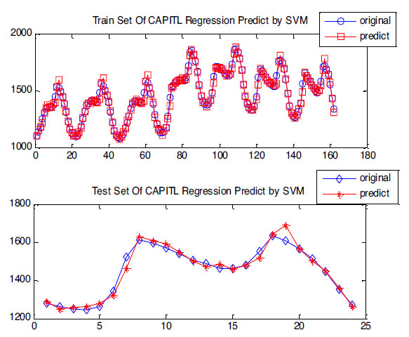 |
Fig. (4). Fitting diagram of predicted SVR value and actual value. |
| - | Parameter | Termination of Algebra | Population Quantity | Best c | g | CVmse |
|---|---|---|---|---|---|---|
| Numerical value | c1=1.5 c2=1.7 | 100 | 20 | 100 | 0.943 | 0.0071 |
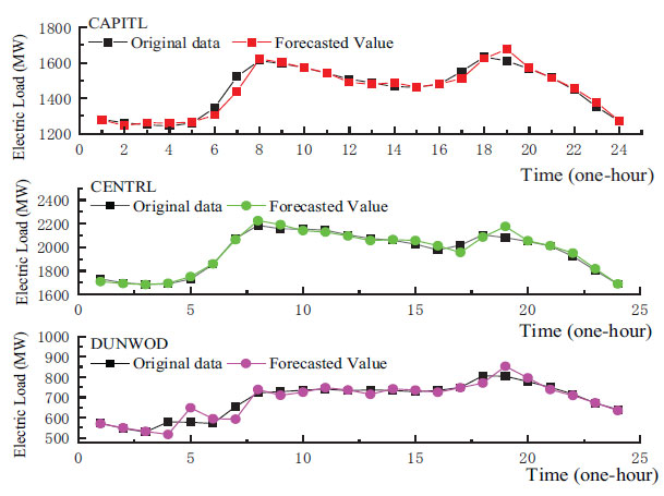 |
Fig. (5). Fitting SVR prediction for three regions. |
 |
Fig. (6). Trend diagram of EMD decomposition variables. |
According to the autocorrelation graph and partial autocorrelation graph after difference and the order, the determination principle is shown in Table 1. The values of p and q were determined to establish the ARIMA (p, d, q) model, and then the ARIMA model was determined by the AIC minimum principle. The optimal ARIMA model established after sequence decomposition of the two regions is shown in Table 2.
The ARIMA model and test indicators (P-value and AIC) of IMF1 and IMF7 combination sequence M1 and IMF2-6 combination sequence M2 in three regions (CAPITL、CENTRL and DUNWOD) are clearly shown in Table 3. According to the optimal model selected by P-value and indicator, AIC as the principle of minimum information, and 24 predicted values in the future were predicted. The predicted values of the two combination sequences were linearly combined through extensive calculations in multiple attempts. Finally, the weighted predicted values were obtained. The fitting results of the predicted value and true value of ARIMA are shown in Fig. (7).
| Model | ACF | d | PACF |
|---|---|---|---|
| AR (p) | hangover | 0 | P order truncation |
| MA (q) | Q order truncation | 0 | hangover |
| ARMA (p,q) | hangover | 0 | hangover |
| ARIMA (p,d,q) | hangover | d | hangover |
| Series Model p 6 12 | AIC | |||
|---|---|---|---|---|
| CAPITL M11 | ARIMA (2,1,1) (0,1,1) | 0.9669 | 0.9704 | 1904.94 |
| CAPITL M21 | ARIMA (3,1,1) (1,1,1) | 0.3056 | 0.6686 | 351.74 |
| CENTRL M12 | ARIMA (2,1,3) (0,1,2) | 0.4143 | 0.0857 | 1519.69 |
| CENTRL M22 | ARIMA (2,1,3) (2,1,1) | 0.8657 | 0.9619 | 794.34 |
| DUNWOD M13 | ARIMA (2,0,2) (1,1,1) | 0.9713 | 0.9898 | 1196.12 |
| DUNWOD M23 | ARIMA (3,1,1) (3,1,1) | 0.0959 | 0.2151 | 412.63 |
Fig. (7) shows the fitting effect of the predicted value and the actual value of the EMD decomposed data based on ARIMA. The sequence is New York City's electric power load and the influencing factors are complicated, which are closely related to the local economy and policies as well as the weather and other natural conditions. Although the time sequence method considers the dependence on the time series and the interference of random fluctuations, it does not have good generalization capability and could not guarantee global optimization. Therefore, it can be seen from the fitting graph of predicted value and actual value that the overall trend is consistent, and the problem of fitting accuracy is not significant.
4. COMPARISON OF MODELS, RESULTS ANALYSIS, AND DISCUSSION
The model is applied to predict the data and then compared with the original power load data to verify the efficiency of the model. In order to further reflect the superiority of this method, this paper chooses the ARIMA model to compare and analyze the power loads of three regions so as to understand the power consumption between regions in depth.
4.1. Selection and Analysis of Comparative Models
In this paper, the power load data of three districts (CAPITL, CENTRL and DUNWOD) from 0:00 on January 1, 2016, to 23:00 on January 8, 2016, were considered. According to the classification and processing of the data, the corresponding model was established, and the power load in the next 24 hours was predicted by the model.
As shown in Fig. (8), based on the power load data of three regions (CENTRL, DUNWOD and CAPITL), the degree of fitting between the actual and predicted values of the four models is compared. As can be seen in the figure, from 0 to 5, the prediction effect of the model is better. This period can be predicted at short intervals based on the previous day's power load. Power load data has short-term stability. The prediction accuracy of the SVR model is not only higher than that of the ARIMA model, but also better than the advanced model (RNN LSTM), which indicates that the prediction accuracy of the SVR model is high, the range of adaptation is large, and it is advanced to a certain extent.
First of all, with respect to the rolling point mechanism changes, SVR can be more flexible in revealing the mechanism of change compared with other models. This is because the SVR can, at some point, extract a flexible power mechanism. It is a kind of very good artificial intelligence algorithms, and handles problems with good comprehensive properties. It not only reduces the risk structure, but the mapping procedure is also simplified. It has higher prediction accuracy than the comparison model. Secondly, the objective model has different effects on different regions, since there is a difference in electricity consumption depending on geographical location and economic development level. It is understood that DUNWOD has a small urban industry and population and limited economic development; therefore, the power load is small, while CENTRL is a central district with a relatively prosperous economy, developed industry and commerce, and more urban residents; therefore, the power load is relatively larger in CENTRL. The CAPITL is a cultural and political capital. In general, the population is small, there is no industry, the economy is dominated by government agencies and tourism, and the electricity load is lower than the CENTRL. Therefore, in addition to better revealing the power mechanism behavior of the CENTRL by SVR, it also provides a more in-depth research direction for the artificial intelligence method. In order to further explain the prediction effect of the model, several quantitative indicators are provided as supplements in this paper.
 |
Fig. (7). ARIMA model prediction effect diagram. |
 |
Fig. (8). Comparison of actual and predicted values of the four models in the three regions. |
table 4-6 show the error data of the three areas. It can be intuitively found that the four prediction error indexes of the other three models are better than that of the ARIMA model. ARIMA model has the most significant prediction error and poor stability. The prediction error of the SVR model is relatively smaller, the stability is good, and the prediction accuracy is high.
First of all, from the perspective of economic development, the regional center of New York City is one of the most active economic markets in the world. It is also one of the most important commercial and financial centers globally, with the most prosperous economic development, having numerous museums, galleries and performing arts competition venues. Therefore, its electricity consumption is relatively larger. In order to adapt to the adjustment of electricity consumption in different industries and departments, the economic effect of electricity consumption fluctuates greatly. Therefore, the error is relatively higher no matter which method is used. Its development is far behind CENTRAL, although DUNWOD is also an important economic and financial center. Secondly, from the perspective of household electricity consumption, CENTRL is the largest and the most crowded city in the United States, with a large number of residents and a huge traffic flow. Therefore, the subway bus has become the primary mode of transportation, which consumes a large amount of electricity. The city of CENTRL is the cultural and political capital home to the House of Representatives and the Senate. Domestic electricity consumption is relatively lower compared to CENTRL for a densely populated city. CENTRL has a distinct climate characteristic with four distinct seasons. Some regions of DUNWOD are not the most suitable places to live due to their unsuitable cold climate and short spring season. Therefore, CENTRL's electricity consumption is still higher, and its fluctuation and error are more significant. Finally, for agriculture and industry in DUNWOD, suitable crops are very limited due to the climatic conditions. However, CENTRL and CAPITL have distinctive climatic characteristics. High agricultural electricity consumption and rapid economic development have restricted the development of the industry. Therefore, CENTRL's electricity consumption is still relatively higher, verifying the size of the above-mentioned error index.
| CAPITL | MSE/*10^4 | RMSE | MAE | MAPE |
|---|---|---|---|---|
| SVR ARIMA |
0.0719 5.9755 |
26.8325 244.4502 |
17.0090 239.9456 |
1.1609 15.9595 |
| RNN | 0.1355 | 36.8115 | 30.9497 | 2.1692 |
| LSTM | 0.1853 | 43.0485 | 35.5544 | 2.4879 |
| CENTRL | MSE/*10^4 | RMSE | MAE | MAPE |
|---|---|---|---|---|
| SVR ARIMA |
0.0886 38.1506 |
29.7699 617.6616 |
21.0903 581.9574 |
1.0498 29.2412 |
| RNN | 1.2603 | 112.2631 | 83.8409 | 4.1508 |
| LSTM | 0.1732 | 41.6257 | 32.0289 | 1.6129 |
| DUNMOD | MSE/*10^4 | RMSE | MAE | MAPE |
|---|---|---|---|---|
| SVR ARIMA |
0.0798 0.9194 |
28.2474 95.8839 |
19.1777 88.2929 |
2.8739 12.5483 |
| RNN | 0.2710 | 52.0649 | 42.2487 | 5.9198 |
| LSTM | 0.2619 | 51.1789 | 40.8439 | 5.8964 |
4.2. Kolmogorov-Smirnov Predictive Accuracy (KSPA) Test
KSPA test is a complementary statistical test method used to distinguish the prediction accuracy of two sets of predictions. It is a non-parametric test based on the Kolmogorov-Smirnov (KS) test principle called the KS prediction accuracy (KSPA) test. The advantage of the KSPA test is that it can not only distinguish the predicted distributions from the two models, but also determine whether the model with the least error also reports the least random error compared to the other model. In addition, the test is not affected by the potential autocorrelation that may exist in the prediction error.
The first part of the KSPA test is the two-sample bilateral KSPA test, which aims to find out that the distribution of the two prediction errors is statistically significantly different (and thus compares the prediction accuracy of the predictions). The second part is the two-sample one-sided KSPA test, which aims to determine whether the prediction with the smallest error based on a loss function also has a random smaller error compared with the competitor's prediction.
The test results of KSPA single-bilateral prediction accuracy are shown in Table 7. First of all, it rejects the null hypothesis because the P-value of the bilateral KSPA test is less than 0.05, which confirms the statistically significant difference between the error of the proposed prediction model and the power load of the comparison model. Secondly, the unilateral KSPA test was used to determine the low random error of the target model and the comparison model. The unilateral KSPA test confirmed that the SVR model, the RNN model, and the LSTM model provided a lower prediction of random error than the ARIMA model, providing additional evidence for the conclusion of the bilateral KSPA test that showed a statistically significant difference between the two predictions.
Figs. (9-11) show the sample prediction error distribution and experience cumulative function distribution of the three cities (CENTRL DUNWOD and CAPITL) obtained by the SVR model, the ARIMA model, RNN model, and the LSTM model, respectively. In this case, we found that the prediction accuracy of SVR is better than that of ARIMA, RNN, and LSTM, and the test results verified the above prediction analysis.
To sum up, the above-tested graphs and models are summarized as follows. As shown in Figs. (9-11), (1) the proposed target model SVR can better describe the random deviation and make the error smaller; (2) The overall advantage of the model and the improvement of prediction accuracy are statistically significant, and (3) The universality and advanced nature of the model are confirmed.
CONCLUSION
Accurate short-term load forecasting is of great significance to the control, operation, and planning of power systems. Based on the non-stationary and random characteristics of power load series, this paper establishes a model and uses 567 power load data from three regions (CAPITL, CENTRL, DUNWOD) from 0:00 on January 1, 2016, to 0:00 on January 8, 2016, to make a prediction analysis of this algorithm. The results are as follows:
| KSPA text | CAPITL/ CENTRL/ DUNWOD | CAPITL/ CENTRL/ DUNWOD |
|---|---|---|
| Two-sided (p-value) | One-sided (p-value) | |
| SVR | <0.01/<0.01/<0.01 | <0.01/<0.01/<0.01 |
| ARIMA | <0.01/<0.01/<0.01 | <0.01/<0.01/<0.01 |
| RNN | <0.01/<0.01/<0.01 | <0.01/<0.01/<0.01 |
| LSTM | <0.01/<0.01/<0.01 | <0.01/<0.01/<0.01 |
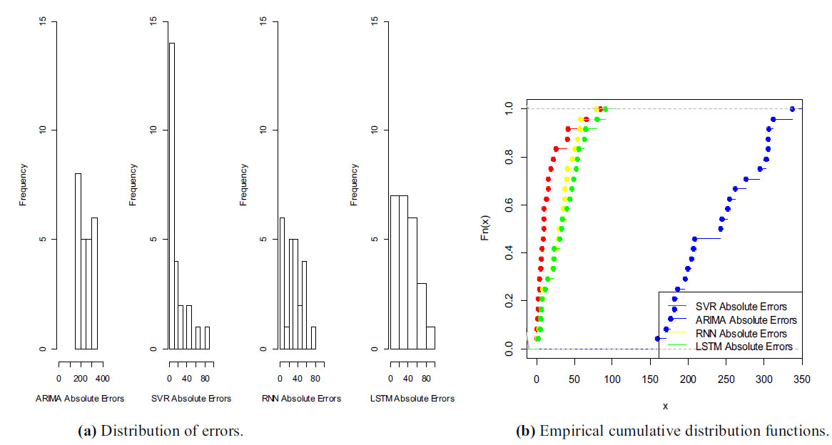 |
Fig. (9). Distribution of errors and empirical cumulative distribution functions of errors in CAPITL. |
 |
Fig. (10). Distribution of errors and empirical cumulative distribution functions of errors in CENTRL. |
 |
Fig. (11). Distribution of errors and empirical cumulative distribution functions of errors in DUNWOD. |
1. Support vector machine regression SVR model mainly has the advantages of linear separability and structural risk minimization. By the decomposition of the EMD method and the combination of each characteristic component, the problem of data fluctuation can be solved effectively, and the superposition of data modes can be eliminated. The modeling analysis of time series eliminates the nonstationarity of power load data and has a good short-term forecasting effect.
2. The prediction accuracy and fitting rate of the support vector machine regression SVR model are better than the ARIMA model. The model can not only objectively, comprehensively, and accurately fit the predicted value of power load, but also adapt to the development needs of modern smart grid and control systems.
3. The proposed model can be widely used in short-term power load production decisions. On the one hand, it can reduce unnecessary waste of electric energy and reduce the cost of power generation while meeting the social demand for electricity. On the other hand, the accurate prediction of power load can not only improve the economic and social benefits, ensure the normal production and life of the society, but also help to maintain the safety and stability of the power grid operation.
CONSENT FOR PUBLICATION
Not applicable.
AVAILABILITY OF DATA AND MATERIALS
Data supporting the findings of the study are available in the article.
FUNDING
Guo-Feng Fan thanks the support from the project grants from Science and Technology of Henan Province of China (No. 182400410419) and the Foundation for Fostering the National Foundation of Pingdingshan University (No. PXY-PYJJ-2016006.
CONFLICT OF INTEREST
The authors declare no conflict of interest, financial or otherwise.
ACKNOWLEDGEMENTS
Guo-Feng Fan thanks the support from the project grants from Science and Technology of Henan Province of China and the Foundation for Fostering the National Foundation of Pingdingshan University.