
RESEARCH ARTICLE
A Many-objective Evolutionary Algorithm Based on Two-phase Selection
Erchao Li1, *, Li-sen Wei1
Article Information
Identifiers and Pagination:
Year: 2021Volume: 1
Issue: 1
E-location ID: e070721194579
Publisher ID: e070721194579
DOI: 10.2174/2666782701666210707144755
Article History:
Received Date: 19/01/2021Revision Received Date: 22/04/2021
Acceptance Date: 24/04/2021
Electronic publication date: 07/07/2021

Abstract
Aims: The main purpose of this paper is to achieve good convergence and distribution in different Pareto fronts.
Background: Research in recent decades has shown that evolutionary multi-objective optimization can effectively solve multi-objective optimization problems with no more than 3 targets. However, when solving MaOPs, the traditional evolutionary multi-objective optimization algorithm is difficult to effectively balance convergence and diversity. In order to solve these problems, many algorithms have emerged, which can be roughly divided into the following three types: decomposition-based, index-based, and dominance relationship-based. In addition, there are many algorithms that introduce the idea of clustering into the environment. However, there are some disadvantages to solving different types of MaOPs. In order to take advantage of the above algorithms, this paper proposes a many-objective optimization algorithm based on two-phase evolutionary selection.
Objective: In order to verify the comprehensive performance of the algorithm on the testing problem of different Pareto front, 18 examples of regular PF problems and irregular PF problems are used to test the performance of the algorithm proposed in this paper.
Method: This paper proposes a two-phase evolutionary selection strategy. The evolution process is divided into two phases to select individuals with good quality. In the first phase, the convergence area is constructed by indicators to accelerate the convergence of the algorithm. In the second phase, the parallel distance is used to map the individuals to the hyperplane, and the individuals are clustered according to the distance on the hyperplane, and then the smallest fitness in each category is selected.
Result: For regular Pareto front testing problems, MaOEA/TPS performed better than RVEA, PREA, CAMOEA and One by one EA in 19, 21, 30, 26 cases, respectively, while it was only outperformed by RVEA, PREA, CAMOEA and One by one EA in 8, 5, 1, and 6 cases. For the irregular front testing problem, MaOEA/TPS performed better than RVEA, PREA, CAMOEA and One by one EA in 20, 17, 25, and 21 cases, respectively, while it was only outperformed by RVEA, PREA, CAMOEA and One by one EA in 6, 8, 1, and 6 cases.
Conclusion: The paper proposes a many-objective evolutionary algorithm based on two phase selection, termed MaOEA/TPS, for solving MaOPs with different shapes of Pareto fronts. The results show that MaOEA/TPS has quite a competitive performance compared with the several algorithms on most test problems.
Other: Although the algorithm in this paper has achieved good results, the optimization problem in the real environment is more difficult, therefore, applying the algorithm proposed in this paper to real problems will be the next research direction.
1. INTRODUCTION
A multi-objective optimization problem contains multiple goals that are optimized at the same time. If the number of optimized goals exceeds 3, it is called Many-objective Optimization Problems (MaOPs) [1]. The objectives of this type of optimization problem are contradictory, and the purpose of optimization is to obtain a set of compromise solutions among multiple objectives. There are many high-dimensional multi-objective optimization problems in the real world, such as vehicle path planning problems [2], automobile crashworthiness design problems [3], active Power Filter [4], etc., which have high theoretical and application value.
Research in recent decades has shown that evolutionary multi-objective optimization can effectively solve multi-objective optimization problems with no more than 3 targets [5]. However, when solving MaOPs, the traditional evolutionary multi-objective optimization algorithm is difficult to effectively balance convergence and diversity. The main difficulties are as follows [5, 6]: First, as the number of targets increases, the Pareto relationship fails, and it is difficult to distinguish between individuals; Second, the number of evolutionary individuals required to approach the Pareto front increases exponentially, which increases the space and time complexity of problem-solving; Third, the search behavior of the population is difficult to investigate, which increases the design difficulty of the change operator. To solve the above problems, the most direct method is to relax the dominance relationship and increase the selection pressure for evolution to the real Pareto front, for example, MFEA [7] based on fuzzy dominance relationship, GrEA [8] based on hypergrid dominance and θ-DEA [9] based on reference vector dominance. However, additional parameter adjustment is required to dominate the area, and inappropriate parameter adjustment will reduce the diversity of the algorithm [10].
An algorithm based on the decomposition idea, which is different from the relaxation of the dominance relationship, decomposes the multi-objective problem into single sub-objectives, generates a uniform weight vector in the space, and uses the aggregation function to select solutions to maintain the convergence and diversity of the population. The most basic decomposition algorithm is MOEA/D [11]. Many algorithms are improved on this framework. Recently, DDEA [12] is proposed, inspired by the classic sorting algorithm quickselect [13], and the individual itself is used as the weight to construct a dynamic decomposition strategy that dynamically adjusts the weight vector to improve the performance of the algorithm, but excessive vector adjustment makes the algorithm unable to balance the convergence and diversity of the algorithm on the problem with regular Pareto front. MaOBSO [14] combines variable classification and decomposition strategies to solve Many-Objective-based problems.
Index-based algorithms use performance index values to represent the quality of the solution in environment selection [15]. Because of its simple and versatile characteristics, it is also a representative method. For example, MOMBIII [16] based on the R2 indicator and MaOEA/IGD [17] based on the IGD indicator, select solutions by obtaining the corresponding indicator values, but a single indicator has a preference in the process of environmental selection, which affects the performance of the algorithm. EIEA [18] adopts the enhanced IGD-NS as the secondary selection criterion in environmental selection. In addition, there are also some algorithms that introduce the idea of clustering to select solutions in the process of environmental selection. Hua Yi cun et al. proposed that CAMOEA [19] introduces hierarchical clustering selection in the critical layer of non-dominated sorting to improve convergence and diversity. Then, Liu Song bai proposed that MaOEA/C [20] pre-divided the population by dividing clusters with the coordinate axis as the clustering center, and then further divided the population by using hierarchical clustering. The algorithm better balances the convergence and diversity, but the solution set cannot achieve good distribution performance on the convex front.
These MaOEAs are proposed to solve MaOPs, however, there are some disadvantages to solving different types of MaOPs. In order to take advantage of the above algorithms, better convergence and distribution in different Pareto fronts are acheived. This paper proposes a many-objective optimization algorithm based on two-phase evolutionary selection. The main contributions of the algorithm are as follows:
1) A two-phase selection algorithm is proposed. In the first phase, a binary scale index is used to screen out a certain difference solution to construct a convergence area and promote the convergence of the population. Especially in the second phase, a hierarchical clustering algorithm based on parallel distance similarity is proposed to perform distributed operations on the constructed regions to maintain the diversity of population.
2) Comparing the algorithm proposed in this paper with four representative many-objective optimization algorithms, the results show that the algorithm can achieve better distribution and convergence when solving problems with regular and irregular Pareto front.
The rest of this paper is organized as follows: Section 2 introduces some related concepts, such as the definition of MaOPs and the ratio based on the indicator. Section 3 presents the details of MaOEA/TPS. The experimental results and discussions are provided in Section 4. At last, our conclusions and future work are presented in Section 5.
2. RELATED CONCEPT
2.1. Concept and Definition of a Many-Objective Optimization Algorithm
Without loss of generality, the minimization problem is taken as an example, generally, a minimize multi-objective optimization problem having n decision variables and m objective variables can be mathematically described as [21]:

where
 is n-dimensional decision vector, Ω represents n-dimension decision space, Y represents an m-dimension objective dimension.
 constitutes m conflicting objective functions and is mapping from n-dimensional decision space Ω to m-dimensional objective space Y. When M is greater than 3, it is called a many-objective optimization problem.
2.2. Radio Based Indicator
Suppose the objective space is
 , the radio-based indicator value
 is defined as follows in Eq. (1):
 |
(1) |
Where
 represents p-norm, literature [15] proved that it is the best indicator when the p is ∞. At the same time, the fitness of xi can be calculated as follows by Eq. (2):
 |
(2) |
If the fitness value of an individual is greater than or equal to 0, it is the necessary and sufficient condition for the individual to be a nondominated solution in the current population. The larger the fitness value is, the more important xi is in the current population.
3. METHODOLOGY
3.1. The Proposed MaOEA/TPS
In this section, our proposed algorithm MaOEA/TPS is introduced thoroughly, which includes the following four subsections. Specifically, the general framework of MaOEA/TPS is provided in Section 3.1. Then, the main algorithmic components of MaOEA/TPS, i.e., the two-phase select strategy, are introduced in Section 3.2.
3.1.1. The Framework of MaOEA/TPS
Algorithm 1 describes the main framework of the proposed algorithm MaOEA/TPS. First, an initial population of size N is randomly generated, and excellent individuals are selected to enter the mating pool. Then, two classical evolutionary operators (the simulated binary crossover (SBX)) and multi-style mutation (PM) are used to generate offspring Qt, merge offspring and parent individuals, and finally select N convergence and diversity from the merged individuals through a two-phase evolutionary selection mechanism; the above steps are repeated until the termination conditions are met. The pseudo code of the overall framework is shown in Algorithm 1:

3.1.2. Two-phase Environmental Selection Strategy
This paper proposes a two-phase evolutionary selection strategy. The specific content is shown in Algorithm 2. The evolution process is divided into two phases to select individuals with good quality. In the first phase, the convergence area is constructed by indicators to accelerate the convergence of the algorithm. In the second phase, the parallel distance is used to map the individuals to the hyperplane, and the individuals are clustered according to the distance on the hyperplane, and then the target and the smallest in each category are selected. Finally, the population that takes into account both convergence and distribution is obtained. The specific operations of each phase are described in detail as follow:

3.1.2.1. Construction of the Convergence Area Based on Radio-Based Indicator
The steps of constructing the convergent region in the first phase are shown in Algorithm 3. The algorithm based on the dominance relationship cannot effectively distinguish individuals. Literature [22] pointed out that the boundary solution can promote the convergence and diversity of the population during the evolution process. But there is a dominant resistance solution in the boundary area, which is very poor on at least one target but is better than other solutions [23]. In order to eliminate the differential solution to protect the boundary solution, the good properties of the indicators in the literature [15] are used to construct the first-phase convergence region. Algorithm 3 has an input Pt (merged individual) and an output Pc (convergence region individual). In line 1, calculate the index value of the merged individual Pt according to formula (1), and then calculate the fitness value of the individual according to formula (2) in line 2. In lines 3-5, when the number of individual index values greater than zero does not exceed N, then sort by the size of the fitness value, and select individuals with high importance directly into the next generation. Otherwise, construct the convergence area based on specific steps in lines 6-16. In lines 7-8, calculate the number of individuals with fitness values greater than zero and calculate the number of individuals to be deleted. In lines 9-13, according to the size of the fitness value, screen out the prescribed number of individuals, lines 14-15, calculate the maximum fmax of each dimension of the remaining individuals, select individuals less than the maximum range for the next phase of optimization, i.e., the area composed of (0,0,0...0) and
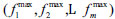 . The schematic diagram of the convergence area is shown in Fig. (1).
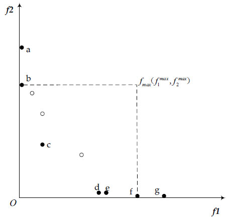 |
Fig. (1). Schematic diagram of convergent region construction. |
As shown in the figure, suppose the size of the population is 5. After crossover mutation, the size of the combined population is 10. Among them, seven individuals with fitness greater than zero are a, b, c, d, e, f, g, and they are all non-dominated solutions. The number of individuals to be deleted is two. a and g are boundary outlier solutions, and their fitness is the smallest in the evolution of the population, and they will be deleted one by one. Next, the maximum value of each dimension is calculated of the remaining individual b, c, d, e, f, that is, the area in the dashed box is the convergence area.
3.1.2.2. Clustering Distribution Selection Based on Parallel Distance
The second-phase distribution operation is shown in Algorithm 4. Generally speaking, a suitable individual similarity measure is very important for clustering. In MaOEA/C [20], the vector angle between individuals was used to measure the similarity, however, it was found that this measurement method is very poor for irregular frontier problems. In order to make the algorithm achieve good distribution on the problem with regular and irregular Pareto front, a clustering distribution selection based on parallel distance similarity is proposed.
Algorithm 4 has an input Pc (the individuals selected in the first phase) and an output C (the collection of population divided after parallel distance clustering). In lines 1-2, parallel distance is used to map the individual Pc after the first phase selection to the hyperplane. Parallel mapping is used to calculate similarity. The distance measurement method can appropriately measure the distance between individuals on different Pareto front shapes. The schematic diagram of parallel distance similarity cluster selection is shown in Fig. (2), and the specific operations are as follows:

First, the individual Pc is normalized, and the individual targets of individual xi are calculated as follows in Eq. (3):
 |
(3) |
Next, the individuals selected in the first phase are mapped to the hyperplane of
 , and the distance calculation formula for any two mapped individuals is as follows in Eq. (4):
 |
(4) |
In the third row, clustering is performed based on the distance calculated by the parallel mapping, and each individual is regarded as a class; K is the number of individuals selected in the first phase. In lines 4-7: cluster the individuals, select the two closest clusters to merge and return to the final cluster when the set conditions are met, otherwise continue to loop. The distance formula between clusters is as follows in Eq. (5):
 |
(5) |
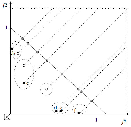 |
Fig. (2). Parallel distance similarity clustering diagram. |

4. RESULTS AND ANALYSIS
This section aims to verify the performance of the MaOEA/TPS algorithm through experimental research. The proposed algorithm was compared with RVEA [24], PREA [15], CAMOEA [19], One by one EA [22] on the problem with regular and irregular Pareto front. All experiments in this article are carried out on a computer with Intel Core, CPU: i5-10400@2.90 GHz, RAM: 16.0 GB. The program is written in Matlab 2016, and runs on the multi-objective optimization algorithm open-source platform PlatEMO-2.7 [25].
4.1. Test Problem and performance Metrics
A total of 18 instances are used to test the performance of the algorithm proposed in this article. They are DTLZ1-2 [26], WFG1-9 [27], and MaF1, 3, 4, 6, 7 [28]. These instances include not only the problems with regular PF (DTLZ1-2, WFG4-9) but also the problems with irregular PF (WFG1-3, MaF1, MaF3, MaF4, MaF6, MaF7). For DTLZ1,the number of decision variables is m-1+5. For DTLZ2, WFG1-2, WFG4-9,the number of decision variables is m-1+10. For WFG3, MaF1, MaF3, MaF4, MaF6, MaF7, the number of decision variables is m-1-10.
In order to evaluate the comprehensive performance of the proposed algorithm, this paper uses two widely used indicators IGD and Spread, accurately and quantitatively. The inverse generation distance is used to comprehensively evaluate the convergence and diversity of the algorithm, and Spread is used to evaluate the distribution of the approximate Pareto front.
(1) IGD [29]: Let P be an approximation set and be a set of non-dominated points uniformly distributed along the true Pareto front, and then the IGD metric is defined as follows:

Where
 is the cardinality of
 ; is the Euclidean distance between
 and its nearest neighbor in P. The smaller the value of IGD, the better convergence and distribution of the approximate solution set and closer to the true Pareto front.
(2) Spread [30, 31]: In order to measure the distribution of the solution, we use the universal indicator Spread. The calculation formula of the indicator is as follows in Eq. (6):

Where
 is the cardinality of P*, P* is the set Pareto optimal solutions, e1, e2, em are m extreme solution in P*.
4.2. Parameter Setting
(1) Population Size: The population sizes are set to be 91, 210, 240, 275, corresponding to m = 3, 5, 8, 10.
(2) Operator: We use a simulated binary crossover (SBX) and polynomial mutation as genetic operators. The crossover probability pc is set to 1.0, and its distribution index
 is set to 20. The mutation probability is set to
 , and n is set to 20.
(3) Comparison algorithm parameter setting: The penalty factor change rate of RVEA is 2, and the reference point adjustment frequency is 0.1.
(4) Number of Runs and termination conditions: All the algorithms in this paper are run on the open-source platform PlatEMO [25]; each algorithm is run independently 20 times, and the standard deviation and average are recorded. When the evaluation times of the objective function reach 30,000 times, the algorithm ends.
(5) Statistical Test: To reach a statistically sound conclusion, the Wilcoxon rank-sum test at the significance level of 0.05 is used to analyze the differences between MaOEA/TPS and the other four algorithms. Symbols “+,” “=”, and “-” indicate the results obtained by other algorithms are better than, similarly to, and worse than that of MaOEA/TPS.
4.3. Comparisons on Problems with Regular Pareto Fronts
In this section, MaOEA/TPS is compared with four representative MaOEAs on problems with regular Pareto fronts. The statistical test results for IGD values and Spread values obtained by the five compared algorithms are summarized in table 1 and 2. In addition, MaOEA/TPS have achieved the most global optimal results on IGD and Spread. Compared with other algorithms, the specific analysis is as follows:
Regarding DTLZ1 with line and muti-model PF, MaOEA/TPS performed best in the cases of 5 objectives, while RVEA was best in the case of 3 objectives and one by one EA obtained the best results in the cases of 8 and 10 objectives. For DTLZ1 and WFG4 with concave PF, MaOEA/TPS only gave a median performance among the compared MaOEAs. Concerning WFG5 with Deceptive PF and WFG6 with muti-modal PF, MaOEA/TPS performed best in the cases of 5, 8, and 10 objectives. In particular, (Fig. 3) shows the IGD convergence curve of the comparison algorithm on WFG5, MaOEA/TPS can quickly stabilize to the minimum, showing the convergence performance of the proposed algorithm on WFG5. In the process of evolution, CAMOEA, PREA, RVEA has similar convergence performance in some cases, and the overall convergence of one by one EA fluctuates greatly. For WFG7 and WFG8 with Uni-modal PF, MaOEA/TPS performed best in the cases of 8, and 10 objectives. Concerning WFG9 with a multi-modal and deceptive PF, MaOEA/TPS performed best in the cases of 5, 8, and 10 objectives; RVEA performed best in the cases of 3 objectives. Fig. (4) shows the convergence curve of the algorithm on WFG9; it shows the performance of the compared algorithms on WFG9. In the case of a small number of targets, CAMOEA, RVEA shows similar performance, but as the number of targets increases, MaOEA/TPS can quickly converge to the best performance index value. In order to intuitively reflect the distribution performance of MaOEA/TPS, (Figs. 5 and 6) presents the nondominated solutions obtained by the compared algorithms on 5-objective WFG6 and 8-objective WFG8. Among these algorithms, MaOEA/TPS has the best solution set distribution, and one by one EA has the worst solution set distribution.
From the one-by-one comparisons in the last row of Table 1, MaOEA/TPS performed better than RVEA, PREA, CAMOEA and One by one EA in 19, 21, 30, and 26 cases, respectively, while it was only outperformed by RVEA, PREA, CAMOEA and One by one EA in 8, 5, 1, and 6 cases, respectively. Therefore, it is reasonable to conclude that MaOEA/TPS showed superior performance over its four competitors in most instances of the regular Pareto front.
4.4. Comparisons on Problems with Irregular Pareto Fronts
In this section, MaOEA/TPS is compared with four representative MaOEAs on problems with irregular Pareto fronts. The statistical test results for IGD values and Spread values obtained by the five compared algorithms are summarized in table 3 and 4. In addition, MaOEA/TPS has also achieved the most global optimal results on IGD and Spread. Compared with other algorithms, the specific analysis is as follows:
Regarding WFG1 with a convex, mixed, and biased PF, MaOEA/TPS performed best in the cases of 3 objectives, while PREA performed best in the cases of 5, 8, and 10 objectives. MaF1 with line and inverted PF, MaOEA/TPS performed best in the cases of 3, 8, 10 objectives. Similarly, (Fig. 7) presents the IGD trajectories of the five compared algorithms on MaF1; MaOEA/TPS shows a good performance on MaF1. Concerning WFG3 with linear and unimodal PF, MaOEA/TPS performed best in the cases of 5, 8, and 10 objectives, while PREA performed best in the cases of 3 objectives. Fig. (8) presents the IGD trajectories of the five compared algorithms on WFG3, and Fig. (9) presents the nondominated solutions obtained by compared algorithms on 5-objective WFG3; they show good performance of MaOEA/TPS in solving WFG3. For WFG2 with a disconnected and mixed PF, MaOEA/TPS performed best in the cases of 3, and 8 objectives, while RVEA performed best in the cases of 5, and 10 objectives. Fig. (10) presents the five compared algorithms on 8-objective WFG2; it shows that MaOEA/TPS can balance convergence and diversity well. Regarding MaF3, it is characterized by a convex PF and a large number of local PFs; only RVEA can solve this problem well. For MaF6 with degenerate PF, MaOEA/TPS performed best in the cases of 8, 10 objectives. For MaF7 with disconnected PF, MaOEA/TPS performed best in the case of 5 objectives.
From the comparisons in the last row of Table 3 MaOEA/TPS performed better than RVEA, PREA, CAMOEA and One by one EA in 20, 17, 25, 21 cases, respectively, while it was only outperformed by RVEA, PREA, CAMOEA and One by one EA in 6, 8, 1, 6 cases. Therefore, it is reasonable to conclude that MaOEA/TPS showed superior performance over its four competitors in most instances of irregular Pareto front.
| Problem | M | D | RVEA | PREA | CAMOEA | One by one EA | MaOEA/TPS |
|---|---|---|---|---|---|---|---|
| DTLZ1 | 3 | 7 | 2.0742e-2 (1.59e-4) + | 2.3329e-2 (4.60e-4) - | 2.2787e-2 (5.24e-4) - | 4.7955e-2 (1.44e-2) - | 2.2173e-2 (3.73e-4) |
| 5 | 9 | 1.1761e-1 (6.47e-2) - | 9.2150e-2 (7.08e-2) - | 8.3818e-2 (3.33e-2) - | 6.8206e-2 (3.69e-3) - | 5.7988e-2 (5.66e-3) | |
| 8 | 12 | 1.5105e-1 (7.65e-2) + | 4.8374e-1 (2.51e-1) + | 1.9419e+1 (5.89e+0) - | 1.0365e-1 (4.55e-3) + | 6.3262e+0 (4.09e+0) | |
| 10 | 14 | 2.2252e-1 (2.27e-1) + | 9.8259e-1 (6.83e-1) + | 3.1184e+1 (1.25e+1) - | 1.1286e-1 (1.31e-2) + | 5.4910e+0 (2.60e+0) | |
| DTLZ2 | 3 | 12 | 5.4498e-2 (1.07e-4) + | 6.0484e-2 (8.42e-4) + | 5.9850e-2 (1.17e-3) + | 5.7085e-2 (8.72e-4) + | 6.1222e-2 (1.00e-3) |
| 5 | 14 | 1.6549e-1 (1.15e-4) + | 1.7265e-1 (1.31e-3) - | 1.7781e-1 (2.98e-3) - | 1.6296e-1 (8.72e-4) + | 1.7107e-1 (1.15e-3) | |
| 8 | 17 | 3.0563e-1 (7.81e-4) + | 3.3482e-1 (1.68e-3) - | 1.1744e+0 (1.22e-1) - | 3.2100e-1 (1.68e-3) + | 3.3097e-1 (1.24e-3) | |
| 10 | 19 | 4.2562e-1 (2.30e-3) - | 4.1923e-1 (2.81e-3) = | 1.2304e+0 (1.07e-1) - | 3.9490e-1 (2.25e-3) + | 4.2253e-1 (1.13e-2) | |
| WFG4 | 3 | 12 | 2.4209e-1 (4.63e-3) = | 2.3877e-1 (4.05e-3) = | 2.4836e-1 (4.47e-3) - | 3.8133e-1 (3.67e-2) - | 2.3966e-1 (4.99e-3) |
| 5 | 14 | 9.6063e-1 (1.95e-3) - | 9.7315e-1 (8.09e-3) - | 9.6812e-1 (7.83e-3) - | 1.4461e+0 (8.30e-2) - | 9.5576e-1 (6.58e-3) | |
| 8 | 17 | 2.8663e+0 (1.81e-2) - | 2.6890e+0 (2.10e-2) - | 2.7608e+0 (2.30e-2) - | 4.0049e+0 (1.95e-1) - | 2.6583e+0 (2.40e-2) | |
| 10 | 19 | 4.4584e+0 (5.51e-2) - | 4.0206e+0 (3.14e-2) = | 4.1067e+0 (3.07e-2) - | 5.8883e+0 (1.31e-1) - | 4.0365e+0 (2.55e-2) | |
| WFG5 | 3 | 12 | 2.3661e-1 (2.30e-3) + | 2.4653e-1 (2.76e-3) = | 2.5122e-1 (4.36e-3) - | 3.7182e-1 (4.82e-2) - | 2.4696e-1 (4.33e-3) |
| 5 | 14 | 9.5117e-1 (1.61e-3) - | 9.6448e-1 (7.66e-3) - | 9.6683e-1 (7.74e-3) - | 1.3993e+0 (8.67e-2) - | 9.4440e-1 (7.75e-3) | |
| 8 | 17 | 2.9063e+0 (3.10e-2) - | 2.7596e+0 (2.92e-2) - | 2.8867e+0 (4.47e-2) - | 4.1798e+0 (1.40e-1) - | 2.6403e+0 (2.68e-2) | |
| 10 | 19 | 4.5187e+0 (6.66e-2) - | 4.0624e+0 (3.14e-2) - | 4.1614e+0 (5.30e-2) - | 6.0814e+0 (1.92e-1) - | 4.0157e+0 (1.89e-2) | |
| WFG6 | 3 | 12 | 2.6525e-1 (1.37e-2) = | 2.5478e-1 (7.91e-3) + | 2.7894e-1 (1.63e-2) - | 5.4192e-1 (6.07e-2) - | 2.6183e-1 (9.32e-3) |
| 5 | 14 | 9.7147e-1 (6.15e-3) - | 9.8767e-1 (8.21e-3) - | 1.0147e+0 (1.36e-2) - | 1.8684e+0 (1.24e-1) - | 9.6389e-1 (7.86e-3) | |
| 8 | 17 | 2.9691e+0 (4.36e-2) - | 2.8529e+0 (2.53e-2) - | 2.9022e+0 (4.59e-2) - | 4.7598e+0 (2.14e-1) - | 2.6605e+0 (2.16e-2) | |
| 10 | 19 | 4.6461e+0 (8.53e-2) - | 4.2078e+0 (5.39e-2) - | 4.2110e+0 (6.89e-2) - | 6.8415e+0 (2.05e-1) - | 4.0714e+0 (2.52e-2) | |
| WFG7 | 3 | 12 | 2.3784e-1 (4.10e-3) = | 2.3984e-1 (4.85e-3) = | 2.4862e-1 (8.01e-3) - | 4.9168e-1 (1.10e-1) - | 2.3863e-1 (4.75e-3) |
| 5 | 14 | 9.6507e-1 (3.03e-3) = | 9.8031e-1 (9.19e-3) - | 9.7205e-1 (7.56e-3) = | 1.8765e+0 (1.70e-1) - | 9.6717e-1 (1.14e-2) | |
| 8 | 17 | 2.9114e+0 (4.07e-2) - | 2.7747e+0 (2.92e-2) - | 2.8965e+0 (5.50e-2) - | 4.3452e+0 (1.59e-1) - | 2.6604e+0 (1.83e-2) | |
| 10 | 19 | 4.2591e+0 (5.67e-2) - | 4.0912e+0 (3.25e-2) - | 4.1715e+0 (4.66e-2) - | 5.9799e+0 (2.33e-1) - | 4.0529e+0 (3.72e-2) | |
| WFG8 | 3 | 12 | 3.1773e-1 (6.35e-3) - | 2.9490e-1 (4.98e-3) + | 3.3353e-1 (5.32e-3) - | 5.7945e-1 (5.32e-2) - | 3.0711e-1 (5.20e-3) |
| 5 | 14 | 1.0162e+0 (3.74e-3) + | 1.0284e+0 (6.36e-3) = | 1.1457e+0 (1.54e-2) - | 1.6236e+0 (1.21e-1) - | 1.0253e+0 (8.32e-3) | |
| 8 | 17 | 3.0609e+0 (2.31e-2) - | 2.9883e+0 (3.26e-2) - | 3.3804e+0 (2.78e-2) - | 4.5489e+0 (2.05e-1) - | 2.7390e+0 (1.69e-2) | |
| 10 | 19 | 4.3744e+0 (5.68e-2) - | 4.2852e+0 (4.17e-2) - | 4.6432e+0 (2.86e-2) - | 6.5967e+0 (4.42e-1) - | 4.1406e+0 (3.79e-2) | |
| WFG9 | 3 | 12 | 2.3076e-1 (4.70e-3) = | 2.3592e-1 (3.47e-3) - | 2.4219e-1 (6.09e-3) - | 3.8052e-1 (4.25e-2) - | 2.3316e-1 (3.82e-3) |
| 5 | 14 | 9.4468e-1 (4.29e-3) - | 9.4441e-1 (9.34e-3) - | 9.9772e-1 (1.30e-2) - | 1.4054e+0 (1.26e-1) - | 9.2792e-1 (8.67e-3) | |
| 8 | 17 | 2.8516e+0 (2.27e-2) - | 2.7330e+0 (1.66e-2) - | 3.2106e+0 (8.88e-2) - | 3.8136e+0 (1.89e-1) - | 2.6584e+0 (2.22e-2) | |
| 10 | 19 | 4.3083e+0 (8.52e-2) - | 4.0003e+0 (3.25e-2) - | 4.5758e+0 (8.47e-2) - | 5.3983e+0 (2.31e-1) - | 3.9099e+0 (3.58e-2) | |
| Best/all | 8/32 | 4/32 | 0/32 | 4/32 | 16/32 | ||
| +/-/= | 8/19/5 | 5/21/6 | 1/30/1 | 6/26/0 | - | ||
Note: ‘+’,’-’and’=’indicate that the result is significantly better, significantly worse and statistically similar to that obtained by MaOEA/TPS, respectively.
| Problem | M | D | RVEA | PREA | CAMOEA | One by one EA | MaOEA/TPS |
|---|---|---|---|---|---|---|---|
| DTLZ1 | 3 | 7 | 1.6179e-2 (4.78e-3) + | 1.6518e-1 (1.79e-2) + | 2.2648e-1 (3.29e-2) + | 1.9644e+0 (5.47e-2) - | 1.2115e+0 (7.38e-1) |
| 5 | 9 | 6.4098e-1 (3.79e-1) + | 1.6646e-1 (1.06e-1) + | 2.0328e-1 (5.15e-2) + | 1.9070e+0 (3.66e-2) - | 1.3957e+0 (4.30e-1) | |
| 8 | 12 | 6.3944e-1 (3.06e-1) - | 3.2094e-1 (1.66e-1) - | 3.7563e-1 (4.18e-2) - | 1.4243e+0 (3.82e-1) - | 1.9110e-1 (1.72e-2) | |
| 10 | 14 | 5.6770e-1 (3.63e-1) - | 6.7697e-1 (2.47e-1) - | 3.4007e-1 (3.06e-2) - | 1.0534e+0 (6.33e-1) - | 1.5962e-1 (1.12e-2) | |
| DTLZ2 | 3 | 12 | 1.7041e-1 (4.10e-4) - | 1.5297e-1 (1.48e-2) + | 2.2959e-1 (2.46e-2) - | 1.4371e-1 (2.89e-2) + | 1.6427e-1 (1.72e-2) |
| 5 | 14 | 1.4901e-1 (1.22e-3) - | 9.9577e-2 (4.53e-3) = | 1.7485e-1 (1.48e-2) - | 8.4573e-2 (1.55e-2) + | 9.9121e-2 (5.23e-3) | |
| 8 | 17 | 7.5384e-2 (4.66e-3) - | 7.8922e-2 (4.38e-3) - | 2.2418e-1 (1.24e-2) - | 6.2386e-2 (2.36e-2) + | 6.7164e-2 (5.67e-3) | |
| 10 | 19 | 1.7084e-1 (6.05e-3) - | 7.4322e-2 (4.84e-3) = | 2.3231e-1 (1.09e-2) - | 5.8964e-2 (1.65e-2) + | 7.7217e-2 (1.42e-2) | |
| WFG4 | 3 | 12 | 2.7112e-1 (1.69e-2) - | 2.3821e-1 (1.74e-2) - | 3.1651e-1 (2.58e-2) - | 3.1483e-1 (2.18e-2) - | 1.7081e-1 (1.61e-2) |
| 5 | 14 | 2.6022e-1 (7.82e-3) - | 2.0307e-1 (1.55e-2) - | 2.3596e-1 (1.79e-2) - | 3.0632e-1 (1.38e-2) - | 1.2147e-1 (8.59e-3) | |
| 8 | 17 | 2.5370e-1 (1.50e-2) - | 2.0138e-1 (1.13e-2) - | 2.2297e-1 (1.94e-2) - | 3.2776e-1 (2.26e-2) - | 1.0613e-1 (7.39e-3) | |
| 10 | 19 | 3.0699e-1 (1.92e-2) - | 2.0065e-1 (1.27e-2) - | 2.0911e-1 (1.38e-2) - | 3.2200e-1 (1.21e-2) - | 1.0042e-1 (5.47e-3) | |
| WFG5 | 3 | 12 | 2.9091e-1 (1.21e-2) - | 2.3717e-1 (1.66e-2) - | 3.0613e-1 (2.95e-2) - | 3.2898e-1 (2.46e-2) - | 1.6700e-1 (1.41e-2) |
| 5 | 14 | 2.6070e-1 (7.35e-3) - | 2.0962e-1 (1.44e-2) - | 2.4377e-1 (1.87e-2) - | 3.1761e-1 (1.37e-2) - | 1.1316e-1 (7.69e-3) | |
| 8 | 17 | 2.6586e-1 (1.70e-2) - | 2.3363e-1 (1.70e-2) - | 2.4716e-1 (1.98e-2) - | 3.2707e-1 (1.81e-2) - | 9.7524e-2 (6.22e-3) | |
| 10 | 19 | 3.6172e-1 (2.00e-2) - | 2.5197e-1 (1.65e-2) - | 2.4652e-1 (1.11e-2) - | 3.1744e-1 (1.39e-2) - | 9.4167e-2 (3.97e-3) | |
| WFG6 | 3 | 12 | 2.7587e-1 (1.85e-2) - | 2.3601e-1 (2.03e-2) - | 3.0923e-1 (3.04e-2) - | 3.3151e-1 (1.88e-2) - | 1.8214e-1 (2.20e-2) |
| 5 | 14 | 2.5784e-1 (8.78e-3) - | 2.2267e-1 (1.72e-2) - | 2.4341e-1 (1.65e-2) - | 2.9157e-1 (9.03e-3) - | 1.0597e-1 (7.02e-3) | |
| 8 | 17 | 2.6694e-1 (1.87e-2) - | 2.5396e-1 (1.64e-2) - | 2.4608e-1 (1.75e-2) - | 2.9536e-1 (1.21e-2) - | 8.9348e-2 (8.79e-3) | |
| 10 | 19 | 3.3478e-1 (2.24e-2) - | 2.6152e-1 (1.74e-2) - | 2.4590e-1 (1.57e-2) - | 2.9095e-1 (1.28e-2) - | 8.9369e-2 (7.46e-3) | |
| WFG7 | 3 | 12 | 2.7896e-1 (1.54e-2) - | 2.4189e-1 (2.30e-2) - | 3.0490e-1 (3.70e-2) - | 3.3268e-1 (2.92e-2) - | 1.7438e-1 (1.97e-2) |
| 5 | 14 | 2.5154e-1 (8.35e-3) - | 2.1186e-1 (1.86e-2) - | 2.4083e-1 (1.50e-2) - | 2.9381e-1 (1.58e-2) - | 1.1320e-1 (7.46e-3) | |
| 8 | 17 | 2.6096e-1 (2.11e-2) - | 2.3473e-1 (1.12e-2) - | 2.3196e-1 (2.13e-2) - | 3.0152e-1 (1.51e-2) - | 9.9773e-2 (6.33e-3) | |
| 10 | 19 | 3.3377e-1 (1.67e-2) - | 2.3407e-1 (1.65e-2) - | 2.3125e-1 (1.96e-2) - | 2.9728e-1 (1.52e-2) - | 9.0472e-2 (5.86e-3) | |
| WFG8 | 3 | 12 | 2.2623e-1 (1.82e-2) - | 2.3447e-1 (1.71e-2) - | 2.7543e-1 (2.57e-2) - | 3.0233e-1 (2.25e-2) - | 1.7485e-1 (1.44e-2) |
| 5 | 14 | 2.4949e-1 (8.47e-3) - | 1.9319e-1 (1.19e-2) - | 2.2360e-1 (1.91e-2) - | 2.4064e-1 (9.92e-3) - | 1.0661e-1 (8.36e-3) | |
| 8 | 17 | 2.5060e-1 (1.80e-2) - | 2.2346e-1 (1.40e-2) - | 2.4130e-1 (1.94e-2) - | 2.5992e-1 (1.77e-2) - | 8.1358e-2 (4.60e-3) | |
| 10 | 19 | 3.8533e-1 (3.90e-2) - | 2.4104e-1 (1.56e-2) - | 2.3882e-1 (1.58e-2) - | 2.4092e-1 (1.40e-2) - | 7.8903e-2 (5.93e-3) | |
| WFG9 | 3 | 12 | 2.8822e-1 (1.96e-2) - | 2.3425e-1 (2.33e-2) - | 3.0624e-1 (2.55e-2) - | 3.2937e-1 (2.15e-2) - | 1.9127e-1 (1.98e-2) |
| 5 | 14 | 2.8833e-1 (9.67e-3) - | 1.9605e-1 (1.27e-2) - | 2.3478e-1 (1.28e-2) - | 3.2245e-1 (1.78e-2) - | 1.2852e-1 (8.58e-3) | |
| 8 | 17 | 2.6034e-1 (1.71e-2) - | 2.0372e-1 (1.29e-2) - | 2.2635e-1 (1.01e-2) - | 3.3999e-1 (2.14e-2) - | 1.0311e-1 (5.34e-3) | |
| 10 | 19 | 3.6460e-1 (2.53e-2) - | 2.0789e-1 (1.55e-2) - | 2.2141e-1 (1.13e-2) - | 3.3300e-1 (1.97e-2) - | 9.9670e-2 (5.44e-3) | |
| Best/all | 1/32 | 1/32 | 0/32 | 4/32 | 26/32 | ||
| +/-/= | 2/30/0 | 3/27/2 | 2/30/0 | 4/28/0 | - | ||
Note: ‘+,’ ’-’ and ’=’ indicate that the result is significantly better, significantly worse, and statistically similar to that obtained by MaOEA/TPS, respectively.
 |
Fig. (3). The IGD trajectories of the five algorithms on WFG5. |
 |
Fig. (4). The IGD trajectories of the five algorithms on WFG9. |
 |
Fig. (5). The objective values of nondominated solutions on 5-objective WFG6. |
 |
Fig. (6). The objective values of nondominated solutions on 8-objective WFG8. |
 |
Fig. (7). The IGD trajectories of the five algorithms on MaF1. |
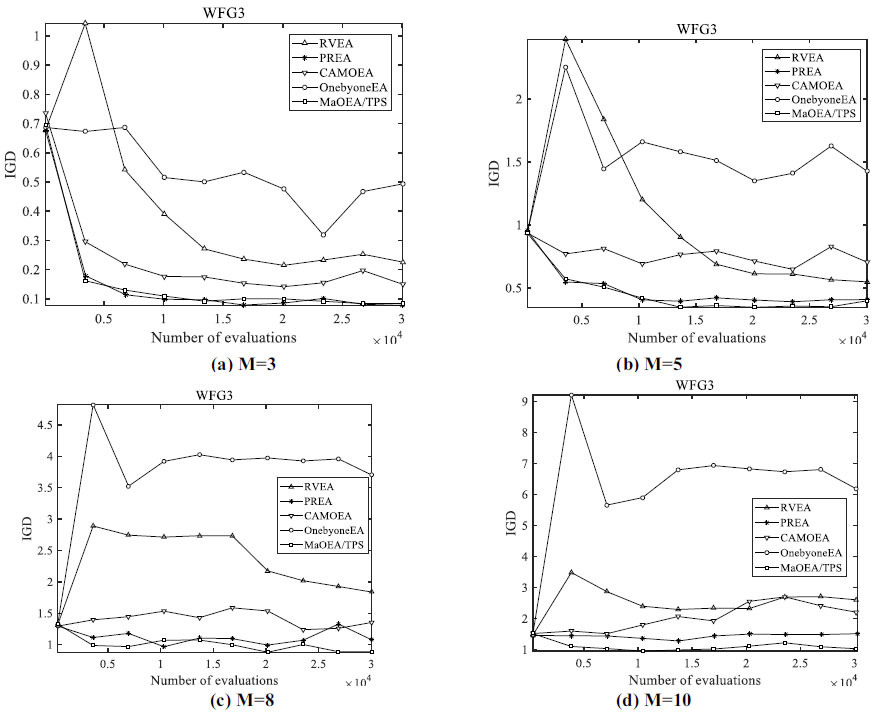 |
Fig. (8). The IGD trajectories of the five algorithms on WFG3. |
 |
Fig (9). The objective values of nondominated solutions on 5-objective WFG3. |
 |
Fig. (10). The objective values of nondominated solutions on 8-objective WFG2. |
| Problem | M | D | RVEA | PREA | CAMOEA | One by one EA | MaOEA/TPS |
|---|---|---|---|---|---|---|---|
| WFG1 | 3 | 12 | 5.1495e-1 (6.94e-2) - | 2.7085e-1 (2.30e-2) = | 4.0345e-1 (4.91e-2) - | 6.1613e-1 (8.67e-2) - | 2.6699e-1 (3.08e-2) |
| 5 | 14 | 1.1968e+0 (9.95e-2) - | 9.8938e-1 (6.20e-2) + | 1.5952e+0 (1.13e-1) - | 1.3495e+0 (8.97e-2) - | 1.0954e+0 (9.82e-2) | |
| 8 | 17 | 1.9805e+0 (1.21e-1) = | 1.6916e+0 (9.40e-2) + | 2.4354e+0 (6.91e-2) - | 2.1993e+0 (1.45e-1) - | 1.9576e+0 (1.22e-1) | |
| 10 | 19 | 2.1524e+0 (1.89e-1) + | 2.1072e+0 (8.55e-2) + | 2.8602e+0 (8.41e-2) - | 2.7038e+0 (1.23e-1) - | 2.5527e+0 (1.39e-1) | |
| WFG2 | 3 | 12 | 1.8966e-1 (6.08e-3) - | 1.8454e-1 (6.28e-3) - | 1.9204e-1 (7.52e-3) - | 2.5495e-1 (1.63e-2) - | 1.7431e-1 (6.09e-3) |
| 5 | 14 | 3.9741e-1 (1.06e-2) + | 4.6202e-1 (1.13e-2) - | 4.9938e-1 (1.18e-2) - | 6.6102e-1 (6.58e-2) - | 4.3155e-1 (1.21e-2) | |
| 8 | 17 | 1.0197e+0 (5.17e-2) = | 1.0473e+0 (2.70e-2) - | 1.1175e+0 (3.07e-2) - | 1.6170e+0 (8.35e-2) - | 9.9454e-1 (2.75e-2) | |
| 10 | 19 | 1.1337e+0 (6.26e-2) + | 1.3702e+0 (4.81e-2) - | 1.3949e+0 (4.53e-2) - | 1.6539e+0 (6.97e-2) - | 1.2212e+0 (4.26e-2) | |
| WFG3 | 3 | 12 | 2.3553e-1 (1.74e-2) - | 8.5441e-2 (7.38e-3) = | 1.6193e-1 (1.21e-2) - | 4.6998e-1 (6.04e-2) - | 8.7803e-2 (8.52e-3) |
| 5 | 14 | 5.3741e-1 (7.65e-2) - | 4.3333e-1 (5.99e-2) - | 7.4480e-1 (8.28e-2) - | 1.4060e+0 (2.24e-1) - | 3.9250e-1 (7.41e-2) | |
| 8 | 17 | 1.9266e+0 (3.53e-1) - | 1.1333e+0 (1.50e-1) - | 1.7264e+0 (1.81e-1) - | 3.7697e+0 (2.94e-1) - | 1.0176e+0 (2.77e-1) | |
| 10 | 19 | 3.0648e+0 (5.25e-1) - | 1.5842e+0 (2.25e-1) - | 2.1758e+0 (2.67e-1) - | 5.4852e+0 (6.61e-1) - | 1.3936e+0 (4.40e-1) | |
| MaF1 | 3 | 12 | 8.2213e-2 (1.73e-4) - | 4.6367e-2 (6.65e-4) - | 4.7819e-2 (9.03e-4) - | 4.5365e-2 (2.57e-3) - | 4.3686e-2 (5.66e-4) |
| 5 | 14 | 2.7201e-1 (1.61e-2) - | 1.1297e-1 (1.33e-3) - | 1.1849e-1 (1.59e-3) - | 1.0192e-1 (2.52e-3) + | 1.0306e-1 (8.13e-4) | |
| 8 | 17 | 4.8857e-1 (6.04e-2) - | 2.0090e-1 (1.83e-3) - | 2.2414e-1 (4.37e-3) - | 4.3575e-1 (2.93e-2) - | 1.8083e-1 (6.67e-4) | |
| 10 | 19 | 5.4334e-1 (7.94e-2) - | 2.3693e-1 (2.84e-3) - | 2.7558e-1 (7.12e-3) - | 4.7175e-1 (2.13e-2) - | 2.1198e-1 (2.00e-3) | |
| MaF3 | 3 | 12 | 3.3282e+1 (3.79e+1) - | 8.2396e-1 (1.75e+0) - | 6.5578e-1 (1.62e+0) - | 4.5234e-1 (6.02e-1) - | 1.6454e-1 (5.06e-1) |
| 5 | 14 | 1.9444e+2 (1.52e+2) - | 3.4347e+1 (2.86e+1) - | 3.7931e+1 (2.30e+1) - | 1.3121e+1 (1.34e+1) = | 1.7278e+1 (1.97e+1) | |
| 8 | 17 | 3.5909e+2 (2.98e+2) + | 5.4900e+2 (4.04e+2) + | 1.7998e+7 (6.29e+7) - | 4.9634e+2 (3.35e+2) + | 8.6620e+4 (3.14e+4) | |
| 10 | 19 | 5.2615e+2 (4.13e+2) + | 3.5400e+3 (2.81e+3) + | 2.2470e+7 (8.54e+7) - | 9.5617e+2 (6.24e+2) + | 1.1856e+5 (5.58e+4) | |
| MaF6 | 3 | 12 | 6.1612e-2 (2.14e-2) - | 5.1449e-3 (1.84e-4) + | 5.2437e-3 (1.36e-4) = | 5.0008e-3 (1.51e-4) + | 5.3736e-3 (2.08e-4) |
| 5 | 14 | 7.9746e-2 (1.34e-2) - | 2.6115e-3 (7.95e-4) = | 2.3794e-3 (6.43e-5) = | 2.1227e-3 (3.43e-5) + | 2.3579e-3 (4.71e-5) | |
| 8 | 17 | 1.5016e-1 (3.58e-2) - | 3.3978e-3 (3.27e-3) - | 2.6407e+0 (2.74e+0) - | 2.1137e-3 (5.98e-5) - | 2.0602e-3 (5.70e-5) | |
| 10 | 19 | 1.0117e-1 (2.63e-2) - | 6.6432e-3 (1.46e-2) - | 7.3535e+0 (3.07e+0) - | 2.9332e-3 (1.46e-4) - | 1.7875e-3 (7.44e-5) | |
| MaF7 | 3 | 22 | 1.0702e-1 (1.57e-3) + | 1.7947e-1 (1.47e-1) - | 6.5957e-2 (1.87e-3) + | 1.0081e-1 (2.26e-2) + | 1.1080e-1 (1.79e-1) |
| 5 | 24 | 5.1802e-1 (1.81e-2) - | 2.3235e-1 (5.89e-2) - | 3.3717e-1 (2.15e-2) - | 3.1570e-1 (3.38e-2) - | 2.0659e-1 (2.62e-3) | |
| 8 | 27 | 1.0117e+0 (6.44e-2) - | 6.1132e-1 (9.78e-3) + | 2.1599e+0 (4.24e-1) - | 1.4129e+0 (2.40e-1) - | 6.7197e-1 (2.03e-2) | |
| 10 | 29 | 1.5970e+0 (3.46e-1) - | 9.7968e-1 (3.76e-2) + | 8.9495e+0 (2.36e+0) - | 2.0773e+0 (3.92e-1) - | 1.0875e+0 (4.35e-2) | |
| Best/all | 4/28 | 6/28 | 1/28 | 4/28 | 13/28 | ||
| +/-/= | 6/20/2 | 8/17/3 | 1/25/2 | 6/21/1 | - | ||
Note: ‘+’ ’-’ and ’=’ indicate that the result is significantly better, significantly worse, and statistically similar to that obtained by MaOEA/TPS, respectively.
| Problem | M | D | RVEA | PREA | CAMOEA | One by one EA | MaOEA/TPS |
|---|---|---|---|---|---|---|---|
| WFG1 | 3 | 12 | 4.5012e-1 (4.32e-2) - | 4.0492e-1 (3.43e-2) = | 4.8154e-1 (3.37e-2) - | 7.8413e-1 (8.10e-2) - | 3.8309e-1 (3.37e-2) |
| 5 | 14 | 5.2629e-1 (4.39e-2) - | 4.0269e-1 (2.66e-2) - | 4.0883e-1 (2.11e-2) - | 6.3073e-1 (4.10e-2) - | 2.8292e-1 (1.64e-2) | |
| 8 | 17 | 9.7563e-1 (7.29e-2) - | 4.0675e-1 (2.87e-2) - | 4.8411e-1 (2.59e-2) - | 8.5599e-1 (1.04e-1) - | 2.6534e-1 (1.22e-2) | |
| 10 | 19 | 1.0180e+0 (1.10e-1) - | 4.2987e-1 (1.55e-2) - | 5.0759e-1 (2.56e-2) - | 9.5686e-1 (7.46e-2) - | 2.6614e-1 (1.18e-2) | |
| WFG2 | 3 | 12 | 3.1275e-1 (3.11e-2) - | 2.8880e-1 (3.50e-2) - | 3.3444e-1 (3.61e-2) - | 5.7329e-1 (2.43e-2) - | 2.3544e-1 (3.34e-2) |
| 5 | 14 | 3.7255e-1 (3.33e-2) - | 3.1897e-1 (2.39e-2) - | 3.2647e-1 (2.04e-2) - | 5.9689e-1 (1.95e-2) - | 2.1401e-1 (2.24e-2) | |
| 8 | 17 | 6.7596e-1 (2.87e-2) - | 3.8129e-1 (2.68e-2) - | 3.9511e-1 (2.43e-2) - | 7.9674e-1 (5.50e-2) - | 1.9857e-1 (1.21e-2) | |
| 10 | 19 | 7.1458e-1 (3.43e-2) - | 4.0592e-1 (2.45e-2) - | 4.3170e-1 (2.22e-2) - | 8.4516e-1 (5.58e-2) - | 1.9622e-1 (1.15e-2) | |
| WFG3 | 3 | 12 | 2.7490e-1 (3.81e-2) - | 2.3847e-1 (2.64e-2) = | 3.1593e-1 (3.15e-2) - | 4.3074e-1 (2.56e-2) - | 2.3219e-1 (2.46e-2) |
| 5 | 14 | 3.8929e-1 (5.11e-2) - | 2.1107e-1 (1.04e-2) - | 2.5379e-1 (1.48e-2) - | 2.3743e-1 (1.67e-2) - | 1.6748e-1 (1.11e-2) | |
| 8 | 17 | 4.1574e-1 (4.81e-2) - | 2.5261e-1 (1.65e-2) - | 2.7987e-1 (1.59e-2) - | 2.5480e-1 (2.95e-2) - | 1.3929e-1 (7.74e-3) | |
| 10 | 19 | 3.7905e-1 (7.61e-2) - | 2.9755e-1 (2.51e-2) - | 3.0542e-1 (1.44e-2) - | 2.5656e-1 (1.86e-2) - | 1.3263e-1 (8.33e-3) | |
| MaF1 | 3 | 12 | 3.2532e-3 (4.09e-3) + | 1.4596e-1 (1.84e-2) + | 2.4855e-1 (1.86e-2) - | 1.7221e-1 (2.80e-2) = | 1.8656e-1 (1.61e-2) |
| 5 | 14 | 5.3797e-1 (5.86e-2) - | 9.5756e-2 (4.59e-3) + | 1.7972e-1 (1.14e-2) - | 1.1335e-1 (1.99e-2) + | 1.3315e-1 (1.43e-2) | |
| 8 | 17 | 9.3607e-1 (6.91e-2) - | 8.1176e-2 (5.89e-3) + | 1.8197e-1 (1.44e-2) - | 2.0432e-1 (4.50e-2) - | 1.3628e-1 (1.42e-2) | |
| 10 | 19 | 1.1658e+0 (2.09e-1) - | 7.5272e-2 (4.27e-3) + | 1.8517e-1 (1.16e-2) - | 1.9792e-1 (2.09e-2) - | 1.2722e-1 (1.55e-2) | |
| MaF3 | 3 | 12 | 1.4684e+0 (6.21e-1) - | 6.0642e-1 (3.66e-1) - | 7.6739e-1 (7.40e-1) - | 1.8939e+0 (2.64e-1) - | 5.7627e-1 (6.20e-1) |
| 5 | 14 | 2.1329e+0 (1.40e-1) - | 1.2514e+0 (2.45e-1) = | 1.2716e+0 (1.64e-1) = | 1.5047e+0 (4.19e-1) - | 1.2943e+0 (4.51e-1) | |
| 8 | 17 | 1.9786e+0 (3.13e-1) - | 1.7334e+0 (3.78e-1) - | 7.6701e-1 (7.89e-2) - | 1.4835e+0 (3.07e-1) - | 3.4635e-1 (5.23e-2) | |
| 10 | 19 | 1.9330e+0 (1.82e-1) - | 1.3897e+0 (1.84e-1) - | 6.7243e-1 (4.84e-2) - | 1.1282e+0 (1.92e-1) - | 2.6483e-1 (2.73e-2) | |
| MaF6 | 3 | 12 | 4.9815e-1 (2.70e-1) - | 2.5090e-1 (2.42e-2) + | 2.8743e-1 (3.61e-2) = | 2.2443e-1 (2.06e-2) + | 2.8117e-1 (2.99e-2) |
| 5 | 14 | 1.5808e+0 (4.37e-1) - | 2.7219e-1 (3.74e-2) + | 3.0858e-1 (2.19e-2) - | 2.2193e-1 (1.57e-2) + | 2.9012e-1 (1.69e-2) | |
| 8 | 17 | 1.2048e+1 (5.16e+1) - | 3.1862e-1 (9.71e-2) = | 5.5871e-1 (3.45e-1) - | 4.3572e-1 (2.03e-1) - | 2.8778e-1 (1.77e-2) | |
| 10 | 19 | -5.7463e+0 (2.75e+1) + | 3.5072e-1 (9.64e-2) - | 4.3320e-1 (7.55e-2) - | 8.6793e-1 (2.11e-1) - | 2.7334e-1 (1.50e-2) | |
| MaF7 | 3 | 22 | 3.4962e-1 (1.53e-2) - | 3.2342e-1 (8.23e-2) - | 3.5114e-1 (2.32e-2) - | 5.5510e-1 (6.36e-2) - | 2.4307e-1 (6.77e-2) |
| 5 | 24 | 3.6472e-1 (4.24e-2) - | 2.5372e-1 (2.34e-2) - | 2.1884e-1 (1.35e-2) - | 3.4641e-1 (1.62e-2) - | 1.6575e-1 (1.02e-2) | |
| 8 | 27 | 4.1089e-1 (5.30e-2) - | 2.4683e-1 (1.12e-2) - | 2.6314e-1 (1.61e-2) - | 3.5965e-1 (3.67e-2) - | 1.0843e-1 (9.44e-3) | |
| 10 | 29 | 5.8251e-1 (8.81e-2) - | 1.0292e-1 (1.97e-2) + | 2.8428e-1 (3.61e-2) - | 2.5495e-1 (5.72e-2) - | 1.2298e-1 (6.71e-3) | |
| Best/all | 2/28 | 5/28 | 0/28 | 2/28 | 19/28 | ||
| +/-/= | 2/26/0 | 7/17/4 | 0/26/2 | 3/24/1 | - | ||
Note: ‘+’,’-’and’=’indicate that the result is significantly better, significantly worse and statistically similar to that obtained by MaOEA/TPS, respectively.
4.5. Comparisons of Running Efficiency
In this section, Table 5 lists the average running time of the five algorithms on each target in order to compare the running time efficiency of each algorithm. RVEA has the shortest running time, followed by one by one EA and CAMOEA, which took less time. PREA and MaOEA/TPS took more time, and MaOEA/TPS was worse than PREA. This is because of the two-stage selection algorithm proposed in this paper, in the first stage, the index method is used to promote the improvement of convergence, and the second stage uses the method based on parallel distance similarity clustering to improve the diversity of the population. They are more time-consuming in the calculation process, which reduces the running time efficiency of MaOEA/TPS.
| Algorithm | 3-objective | 5-objective | 8-objective | 10-objective |
|---|---|---|---|---|
| RVEA | 1.09e+00 | 9.21e-01 | 9.60e-01 | 1.02e+00 |
| PREA | 1.82e+00 | 2.75e+00 | 9.07e+00 | 1.50e+01 |
| CAMOEA | 1.40e+00 | 1.44e+00 | 1.88e+00 | 1.88e+00 |
| One by one EA | 1.29e+00 | 1.49e+00 | 1.81e+00 | 2.33e+00 |
| MaOEA/TPS | 5.46e+00 | 1.80e+01 | 3.41e+01 | 4.90e+01 |
CONCLUSION AND FUTURE WORK
The paper proposes a many-objective evolutionary algorithm based on two-phase selection, termed MaOEA/TPS, for solving MaOPs with different shapes of Pareto fronts. The convergence area is constructed through indicators to improve the convergence ability of the algorithm in the first phase of the algorithm, and then individuals are selected through clustering based on parallel distance similarity to obtain a uniformly distributed solution set in the second phase of the algorithm. The algorithm is compared with RVEA, PREA, CAMOEA, one by one EA on the problem with regular Pareto PF and irregular Pareto PF. The results show that MaOEA/TPS has quite a competitive performance compared with the several algorithms on most test problems. Although the algorithm in this paper has achieved good results, the optimization problem in the real environment is more difficult, therefore, applying the algorithm proposed in this paper to real problems will be the next research direction.
ETHICS APPROVAL AND CONSENT TO PARTICIPATE
Not applicable.
HUMAN AND ANIMAL RIGHTS
No Animals/Humans were used for studies that are the basis of this research.
CONSENT FOR PUBLICATION
Not applicable.
AVAILABILITY OF DATA AND MATERIALS
The authors confirm that the data supporting the results and findings of this study are available within the article.
FUNDING
The work is partially supported by the National Natural Science Foundation of China (62063019,61763026), the Natural Science Foundation of Gansu Province (20JR10RA152).
CONFLICTS OF INTEREST
The authors declare no conflict of interest, financial or otherwise.
ACKNOWLEDGEMENTS
The authors are very grateful to Yuyan Mao and Yang Zhou for their help in algorithm design.