
RESEARCH ARTICLE
Multi-objective Evolutionary Algorithm based on Two Reference Points Decomposition and Historical Information Prediction
Er-chao Li1, *, Kang-wei Li1
Article Information
Identifiers and Pagination:
Year: 2021Volume: 1
Issue: 1
E-location ID: e060821195348
Publisher ID: e060821195348
DOI: 10.2174/2666782701666210806100730
Article History:
Received Date: 19/01/2021Revision Received Date: 12/04/2021
Acceptance Date: 27/04/2021
Electronic publication date: 06/08/2021

Abstract
Aims: The main goal of this paper is to address the issues of low-quality offspring solutions generated by traditional evolutionary operators, as well as the evolutionary algorithm's inability to solve multi-objective optimization problems (MOPs) with complicated Pareto fronts (PFs).
Background: For some complicated multi-objective optimization problems, the effect of the multi-objective evolutionary algorithm based on decomposition (MOEA/D) is poor. For specific complicated problems, there is less research on how to improve the performance of the algorithm by setting and adjusting the direction vector in the decomposition-based evolutionary algorithm. Considering that in the existing algorithms, the optimal solutions are selected according to the selection strategy in the selection stage, without considering whether it could produce the better solutions in the stage of individual generation to achieve the optimization effect faster. As a result, a multi-objective evolutionary algorithm based on two reference points decomposition and historical information prediction is proposed.
Objective: In order to verify the feasibility of the proposed strategy, the F-series test function with complicated PFs is used as the test function to simulate the proposed strategy.
Methods: Firstly, the evolutionary operator based on historical information prediction (EHIP) is used to generate better offspring solutions to improve the convergence of the algorithm; secondly, the decomposition strategy based on ideal point and nadir point is used to select solutions to solve the MOPs with complicated PFs, and the decomposition method with augmentation term is used to improve the population diversity when selecting solutions according to the nadir point. Finally, the proposed algorithm is compared to several popular algorithms by the F-series test function, and the comparison is made according to the corresponding performance metrics.
Results: The performance of the algorithm is improved obviously compared with the popular algorithms after using the EHIP. When the decomposition method with augmentation term is added, the performance of the proposed algorithm is better than the algorithm with only the EHIP on the whole, but the overall performance is better than the popular algorithms.
Conclusion: The experimental results show that the overall performance of the proposed algorithm is superior to the popular algorithms. The EHIP can produce better quality offspring solutions, and the decomposition strategy based on two reference points can well solve the MOPs with complicated PFs. This paper mainly demonstrates the theory without testing the practical problems. The following research mainly focuses on the application of the proposed algorithm to practical problems such as robot path planning.
1. INTRODUCTION
The multi-objective evolutionary algorithm based on decomposition [1] decomposes a multi-objective optimization problem (MOP) [2] into a set of single-objective optimization problems by setting a set of uniformly distributed reference vectors. When solving the MOPs, especially high-dimensional MOPs, MOEA/D shows good results in convergence and distribution. This multi-objective evolutionary algorithm based on decomposition has been recognized as a promising method for solving simple MOPs, but for some complicated MOPs, the effect of MOEA/D is poor [3]. For specific complicated problems, there is less research on how to improve the performance of the algorithm by setting and adjusting the direction vector in the evolutionary algorithm based on decomposition [4, 5]. Based on this, in order to improve the ability of MOEA/D to solve the MOPs with complicated PFs, Qi et al. [6] proposed a multi-objective evolutionary algorithm based on decomposition with adaptive weight adjustment, where a new initialization method of weight vectors to generate the initial set of weight vectors is introduced. The algorithm used an adaptive weight vector adjustment strategy to detect overcrowded solutions on PFs at the solution selection stage and then adjust the weight vectors at more crowded solutions to where the solutions are sparse as a way to ensure distribution of population. This algorithm increases the computational complexity because the weight vectors have to be adjusted continuously. Wang et al. [7] studied the influence of reference point setting on the selection of solutions in evolutionary algorithms based on decomposition. In order to balance diversity and convergence, a new MOEA/D based on ideal point and nadir point was proposed, and an improved global replacement strategy was used to enhance the performance in individual selection. In this algorithm, the whole population is first normalized to two sets according to ideal point and nadir point, and then solutions are selected in different sets according to different weight vectors, which effectively improved the diversity of the population but still had shortcomings in terms of convergence. V. Ho-Huu et al. [8] proposed an improved MOEA/D (iMOEA/D) for the bi-objective optimization problem in order to solve the practical application problems of PF with a long tail or a sharp peak, which usually has complicated characteristics. To demonstrate the performance of iMOEA/D, it is applied to the optimal design problem of the truss structure. In iMOEA/D, the set of weight vectors defined in MOEA/D is numbered and divided into two subsets: one is the set of odd weight vectors, and the other is the set of even weight vectors. Then a two-stage search strategy based on the MOEA/D framework is proposed to optimize the corresponding populations. In addition, an adaptive substitution strategy and a stopping criterion are introduced to improve the overall performance of iMOEA/D. The multi-objective evolutionary algorithm based on decomposition with two reference points can effectively enhance the diversity of the populations, but the convergence is still insufficient.
In order to further improve the convergence, Bi et al. proposed an improved NSGA-III [9] algorithm based on elimination operator (NSGA-III-EO) [10] based on Nondominated Sorting Genetic Algorithms III (NSGA-III). In this algorithm, firstly, the reference points with the maximum number of niches are identified by the elimination operator. Then the relevant individuals are ranked using the penalty-based boundary intersection (PBI). In the process of selecting solutions to ensure convergence, the method of eliminating poorer individuals is used instead of the method of selecting better individuals. This algorithm can better improve convergence and evolutionary efficiency. Wu et al. [11] proposed a multi-objective evolutionary algorithm based on adversarial decomposition. This algorithm utilizes the complementary characteristics of different scalarizing functions in a single paradigm, and the diverse population and the convergence population are introduced to co-evolve. In order to avoid allocating redundant computing resources to the same area of PF, the two populations are matched into one-to-one solution pairs on PF according to their working areas. In the process of selection, each solution pair contributes at most one main mating parent node. This algorithm also has great advantages in balancing convergence and diversity. Liang et al. [12] proposed a two-round environment selection strategy to seek a good compromise between diversity and convergence of the population. In the first round, the solutions with smaller neighborhood densities are selected to form a candidate pool, in which the neighborhood density of solutions is calculated based on a new adaptive location transformation strategy. In the second round, the solutions with the best convergence are selected from the candidate pool and inserted into the next generation. This process is repeated until a new population is generated. The two-round selection strategy works well in balancing population diversity and convergence, but it still has significant limitations for solving complex irregular optimization problems.
All the above algorithms select the optimal solution based on the selection strategy in the selection stage without considering whether a better solution can be generated in the individual generation stage to facilitate optimization. In contrast, in the dynamic multi-objective optimization algorithm [13-15], the PF of the next environment can be predicted based on the PF in the historical environment when the environment changes. In view of this, considering that the historical solution set may have some guiding effect on the generation of new solutions, in this paper, we introduce historical information [16] and generate the next-generation solutions according to the corresponding prediction model, and combine it with two reference point decomposition method to solve the MOPs with complicated PFs.
Based on the above analysis, this paper proposes a multi-objective evolutionary algorithm based on two reference points decomposition and historical information prediction. In order to improve convergence, in this algorithm, a certain set of historical solutions is retained, and the prediction model is combined with differential evolution by introducing an evolutionary operator based on historical information prediction (EHIP) to generate new solutions with better quality; to improve diversity, the solutions are selected using a decomposition strategy with two reference points, the ideal point and the nadir point [17], and the augmented achievement scalarizing function (ASF) with an enhancement term is used in the selection of solutions based on the nadir point.
The rest of the paper is organized as follows. Second half of section 1 contains background knowledge of the theoretical basis of the research. Section 2 presents the details of the proposed strategies and the proposed algorithm. Section 3 contains the analysis of experimental results. Section 4 contains the conclusions.
1.1. Basic Concepts
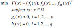
There are two kinds of multi-objective optimization algorithm [18]: maximizing objective function value and minimizing objective function value. Here, minimizing objective function value is taken as an example in Eq. (1):
 |
(1) |
Where
 is n-dimensional decision variable, Ω is the feasible search region,
 is a M-dimensional vector of objective functions, and
 is the objective space,
 are p inequality constraints,
 are q equality constraints. In the following, several definitions of Pareto domination [19, 20] are given.
Pareto domination: for any two solutions
 , if
, if
 for
for
 is said to dominate
 .
.
Pareto optimal solutions: let
 , if there does not exist
 satisfying, p y x, x is called Pareto optimal solution.
The set of Pareto optimal solutions: composed by all Pareto optimal solutions, which can be defined as:

Pareto front: It is the images of the objective function values corresponding to the solutions of PF, which can be defined as

ideal point: a point
 is called the ideal point if

nadir point: a point
 is called the nadir point if

 |
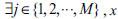
Fig. (1). Pareto optimal points obtained based on
|
 respectively.
1.2. Research Motivation
1.2.1. Decomposition Method based on Two Reference Points
Multi-objective evolutionary algorithm based on decomposition can produce a group of uniform weight vectors; each weight vector corresponds to a solution, so the optimal solution is uniformly distributed with the weight vectors. However, the multi-objective evolutionary algorithm based on decomposition shows its shortcomings when solving optimization problems with extremely irregular PF. As shown in Fig. (1a), when the PF is extremely convex, and the weight vector passing through the ideal point is used, the optimal solutions generated according to the weight vectors have regular distribution. However, it shows that the situations in the middle are dense, and the situations in the boundary are sparse. Similarly, as shown in Fig. (1b), when the PF is extremely convex, and the weight vector passing through the nadir point is used, it shows the situations that in the middle are sparse and the situations in the boundary are dense. As shown in Fig. (2), when the nadir point is introduced, according to the decomposition of the weight vector passing through the nadir point, the situation is just complementary to the situation passing through the ideal point; thus combining the two reference points will effectively solve this situation. Therefore, this paper introduces the ideal point and the nadir point to solve the complex multi-objective optimization problem with an irregular front.
In this paper, the Das and Dennis system scheme decomposition technique [21] is used to generate a set of uniformly distributed reference points on the unit hyperplane, and the vectors from the origin to the reference points form the weight vectors. The number of reference points is shown in Eq. (2).
 |
(2) |
Where N is the number of reference points, H is a parameter, and M is the dimension of the objective, the sum of all elements in
 is 1, and each dimensional element of w is in
 .
.
2. METHODS
2.1. The Proposed MOEA/D-EHIP-ASF
In this section, we proposed a multi-objective evolutionary algorithm based on two reference points decomposition and historical information prediction, and we call this algorithm MOEA/D-EHIP-ASF. Next, the proposed algorithm is introduced in detail.
 |
Fig. (2). Pareto optimal points obtained based on both
|
2.1.1. Initialization
(1). Initialize Weight Vectors
According to Das and Dennis system scheme decomposition technology, two groups of weight vectors are initialized. The directions of the two groups of weight vectors are the same. One group passes through the ideal point, and the other group passes through the nadir point. The neighborhood of two groups of weight vectors is calculated according to Euclidean distance, which is used for the evolutionary operation to generate new solutions, where the set of the neighborhood is represented by B.
(2). Initial Population
The decision variables of each solution in the population are obtained by random sampling in the decision space. After the initial population is obtained, the population is divided into two populations, which evolve according to the ideal point and the nadir point, respectively. In order to initialize the ideal point and the nadir point, we first need to sort the initial population to get the non-dominated solutions set NP. The ideal point and the nadir point are
 and
and
 , respectively.
2.1.2. Normalization
Since many MOPs have different ranges of PFs, in order to facilitate the processing of objective function values with different ranges of PFs in the same range, the objective values of all solutions in the population need to be normalized before optimization. For each solution x, the calculation formula of the normalized objective function value is calculated in Eq. (3) as follows:
 |
(3) |
No matter which weight vectors is used, the whole population is normalized according to the ideal point.
2.2. Evolutionary Operator based on Historical Information Prediction
With the increase of the number of iterations, the quality of the solutions in the population will be better and better, and the solutions in the population will be closer to the real front. In the traditional evolutionary algorithm, only the contemporary optimal solutions are retained as the selection pool for evolutionary operation, and the historical solution sets of each previous generation are discarded. In fact, the historical solution sets of previous generations can reflect the convergence direction of the Pareto solution set to the real front to a certain extent, so the historical information can be used to guide the individuals to a better direction to predict the next generation of individuals. The multi-objective evolutionary algorithm based on decomposition generates a better solution in the direction of the weight vector to replace the solution of the previous generation in each iteration, so the next generation solutions can be considered to be predicted based on historical information in the direction of the weight vectors.
The optimal solutions associated with each weight vector at each iteration can form a sequence [22]:
 denotes the solution associated with the i-th weight vector when the current iteration number is k. this sequence can reflect the rule of change of the optimal solutions associated with a certain weight vector to the real solutions. The prediction of the solution associated with the i-th weight vector in the (k+1)-th iteration can be expressed in Eq. (4) as follows:
 |
(4) |
Where f is the model for predicting the next-generation solutions. In this paper, the Prem model proposed by Aimin Zhou is used to predict the problem that the Pareto optimal solutions change linearly. The new individuals predicted are expressed as follows in Eq. (5):
 |
(5) |
Where t is the step size and follows the normal distribution as represented in Eqs. (6 and 7)).
 |
(6) |
As shown in Fig. (3), The solid black circles represent the best individuals of the present generation, the hollow circles represent the best individuals of the previous generation, and the triangles represent the next generation of individuals generated by the evolutionary operator based on historical information prediction. The red arrow indicates the evolutionary direction of the individuals on the corresponding weight vectors. In general, the shape of PF is relatively simple in the objective space. With the increase of the number of iterations, the change direction of PF can be known generally, which is basically moving to the real PF. However, the shape of PS in the decision space is complex and unknowable, and the movement direction of PS is more complicated. When the step size is small, it can be approximately considered that PS moves linearly toward the real PS with the increase of the number of iterations according to the differential principle, while the pattern of PS movement cannot be accurately predicted when the step size is large.

 |
Fig. (3). Distribution of solutions predicted by the evolutionary operator. |
In this paper, we proposed an evolutionary operator based on historical information prediction (EHIP) by combining the prediction of solutions based on historical information with the original differential evolutionary (DE) [23] and adding a scaling factor to the prediction term to increase its accuracy. In order to increase the diversity, we add the contemporary population information, that is, horizontal information, to avoid falling into local convergence. The expression of EHIP is generated in Eqs. (8 and 9)) as follows:
 |
(8) |
Where
 is horizontal information, F is the control parameter of differential evolution, E is scaling factor, CR is crossover probability.
 are the j-th and h-th solutions selected from the current mating pool.
 is the r-th decision variable of the solution in the (k+1)-th iteration generated by the evolutionary operator.
2.3. Decomposition Approach of Two Reference Points
2.3.1. Tchebycheff Decomposition Approach
Among many approaches of decomposing MOPs into a set of scalar optimization subproblems [24, 25], the penalty-based boundary intersection (PBI) approach can effectively solve the MOPs with convex PFs, while Tchebycheff (TCH) decomposition approach has an obvious effect on the MOPs with non-convex PFs. The TCH decomposition approach based on can be defined as follows in Eq. (10):
 |
(10) |
Where w is the weight vector of the corresponding subproblem, it can be expressed as follows in Eq. (11):
 |
(11) |
TCH decomposition approach based on
 can be defined as follows in Eq. (12):
 |
(12) |
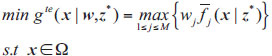
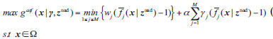
2.3.2. ASF Decomposition Approach
The ASF decomposition approach based on
can be defined as follows in Eq. (13):
 |
(13) |
The difference between ASF and TCH is that ASF uses the
instead of the
 , and increases the augmentation term, α is the augmentation coefficient. The augmentation term in ASF can increase the non-dominated strength of the solutions. When is zero, ASF is the same as TCH. The schematic diagram of the ASF decomposition approach is shown in Fig. (4).
 |
Fig. (4). ASF decomposition approach. |
As shown in Fig. (4), the area surrounded by a black dotted line and coordinate axis is the area dominated by F(x) when α is greater than zero, and the area surrounded by a red dotted line and coordinate axis is the area dominated by F(x) when α is equal to zero. It can be clearly seen from the figure that the area dominated by F(x) is larger when is greater than zero. Therefore, when α is greater than zero, F(x) dominates F(y), so the search range can be expanded.
2.4. Decomposition of Subproblems
The whole population is decomposed into N subpopulations according to the angle between the weight vectors and each individual. Each subpopulation corresponds to the Tr weight vectors closest to its angle, and then only the individuals closest to each weight vector are found as the individuals in each subpopulation, and the subpopulation corresponding to the two reference points is divided in the way shown in Eq. (14).
 |
(14) |
Where
 denotes the normalized objective function value of the individual nearest to the corresponding weight vector, and v is the predefined weight vector, which is taken as w and γ depending on the weight vector as well as the reference point, respectively. In the whole population,
 is the angle between
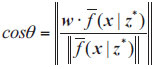
 and wi, and Ci is the subpopulation composed of the i-th vector vi and its solutions with the smallest angle. The angle is calculated by the absolute value of cosine value to ensure consistency with the change of the angle, and its calculation formula is given as follows in Eq. (15):
 |
(15) |
Similarly, when the weight vector is γ, the calculation formula is given as follows in Eq. (16):
 |
(16) |
The principle of the objective space decomposition method based on an angle is shown in Fig. (5). As shown in the figure, any two weight vectors wi and wj are selected, and six different individuals are distributed around them. In the traditional multi-objective evolutionary algorithm, the calculation method based on Euclidean distance is generally used to find the individuals associated with the weight vector. For example, in the process of decomposition, only x2 and x4 are divided into the same interval according to Euclidean distance. This decomposition method improves the convergence of the algorithm but has some defects in maintaining diversity. When using the decomposition strategy of angle-based objective space to divide the subspace, not only x2 and x4 but also x6 are included in the same subinterval, which will maintain the diversity of the population to a great extent in the process of selecting solutions.
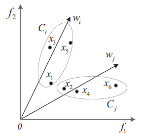 |
Fig. (5). Decomposition method of objective space based on angle. |
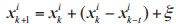
2.5. Global Selection Strategy
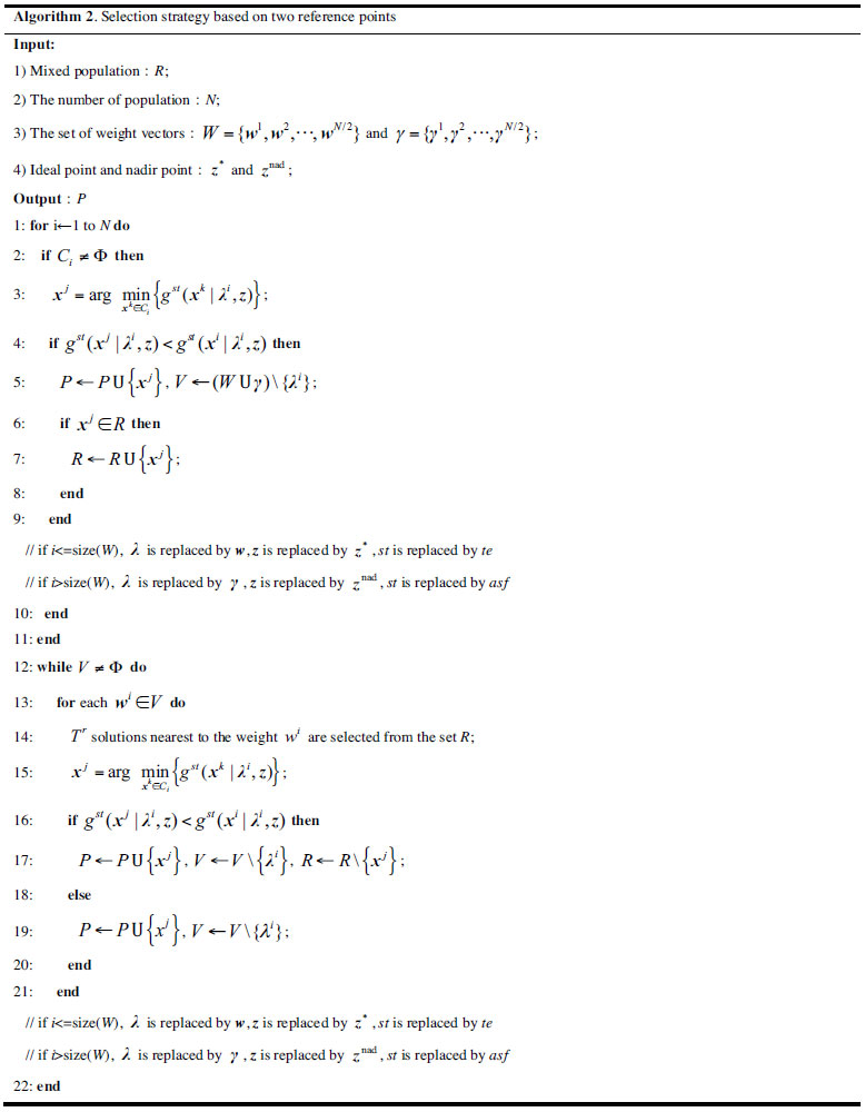
In the process of solution selection, the population is divided into two parts, the first half corresponds to the ideal point, and the TCH decomposition approach based on the ideal point is used to select the solutions; the second half corresponds to the nadir point, and the ASF decomposition approach based on the nadir point is used to select the solutions. Because there is no nearest individual around the weight vector when the individual is associated, the weight vector which is not associated with the individual is put into the set V. At this time, the neighborhood individual of the weight vector is found and selected until it has a corresponding solution, it is removed from the set V. Set P stores the optimized individuals, while set R stores the non-optimized individuals. The pseudo-code of the selection strategy based on two reference points is presented in algorithm 2.
3. RESULTS AND DISCUSSION
All experiments in this paper were implemented using Matlab codes and run on a personal computer having an Intel(R) Core(TM) i5-10400 CPU, 2.90 GHz (processor), and 8.00 GB (RAM).
3.1. Benchmark Problems
This chapter uses F series problems as test functions, which are shown in Table 1. The PSs of the three multi-objective optimization problems F1, F2, and F3 are linear and unimodal [26], and their PFs shapes are complicated. The distribution range of PF in each dimension of F1 is quite different, and one dimension is ten times the other dimension. The PF of F2 is a very convex linear curve with two segments. The PF of F3 is concave in part and convex in part. These three test functions test the ability of the algorithm to deal with problems of complex PFs. The PSs of F4 and F5 are unimodal, indivisible, and complicated. The convergence degree of solutions of two test problems is different, and the solutions of the boundary are more difficult to converge than the middle. F6 and F7 are two multimodal multi-objective optimization problems with complicated PSs shapes. The PSs of F8 and F9 are unimodal, indivisible, and complicated. The PFs of the two test problems is an inverted triangle.
In order to verify its feasibility, it is compared with the classical algorithms MOEA/D-MR, MOEA/D-DE [27], NSGA-III-EO, 2REA and MOEA-TDA [28].
3.2. Parameter Settings
The population size and number of calculations were kept the same for all algorithms to ensure a fair comparison. The crossover probability CR is 1.0, the control parameter of differential evolution F is 0.45, and the scaling factor E is 0 when the number of calculations was less than 10*N; otherwise, E is 0.05 and δ is 0.8. All algorithms were calculated 150,000 times on each test function and run 20 times independently. The test function parameters are set as shown in Table 2.
3.3. Performance Metrics
In order to demonstrate the performance of the algorithm more accurately, we usually need to make a quantitative comparison. In order to evaluate the convergence and diversity, we use the convergence metric GD [29] and diversity metric DM [30] as the Performance metrics, respectively. In order to evaluate the comprehensive performance, we use the more widely used comprehensive performance metrics IGD [31] and HV [32].
1) Generational Distance (GD): It was proposed by Van and Lamont, which represents the average distance from the optimal solutions set to the real Pareto front. It is computed by Eq. (17).
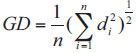 |
(17) |
Where n is the number of standard points selected from the real Pareto front and di is the minimum Euclidean distance between the i-th individual in the optimal solutions set and the real Pareto front. It is noted that the method with a lower GD metric is better.
2) Diversity Metric (DM): The principle of the diversity metric is to project the non-dominated points obtained by each generation onto a suitable hyperplane, thus losing one dimension of the points. The hyperplane is divided into many small grids, and the diversity metric is defined depending on whether each grid contains a non-dominated point. If all the grids are represented by at least one point, it means the best possible diversity measure is achieved. If some grids are not represented by a non-dominated point, the diversity is poor. It is computed by Eqs. (18-20).
 |
(18) |
| Test Function | Function Expression | Constraint Condition |
|---|---|---|
| F1 |

|

|
| F2 |
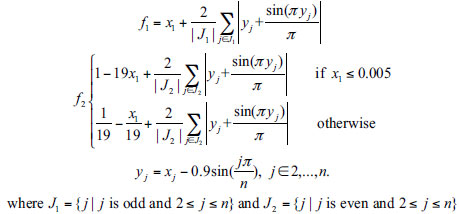
|

|
| F3 |

|

|
| F4 |

|

|
| F5 |

|

|
| F6 |

|

|
| F7 |

|

|
| F8 |

|

|
| F9 |

|

|
| Test Function | Dimension of target (M) | Dimension of decision variable (D) | Population size(N) |
|---|---|---|---|
| F1~F7 | 2 | 30 | 200 |
| F8~F9 | 3 | 10 | 600 |
 |
(20) |
The value of m(h(i,j…)) corresponding to h(i,j…) is shown in the Table 3. H(i,j…) is the same as h(i,j…).
| h(…j-1…) | h(…j…) | h(…j+1…) | m(h(…j…)) |
|---|---|---|---|
| 0 0 1 0 1 0 1 1 |
0 0 0 1 1 1 0 1 |
0 1 0 1 0 0 1 1 |
0.00 0.50 0.50 0.67 0.67 0.75 0.75 1.00 |
P* is a set of reference points obtained by uniform sampling on the real Pareto front, P is a set of approximate optimal solutions obtained by using the evolutionary algorithm, and F is the set of non-dominated P* in the P. It is noted that the method with a larger DM metric is better.
3) Inverse Generation Distance (IGD): IGD takes into account the convergence and diversity of the optimal solutions set. It is calculated by the average distance between a set of reference points uniformly sampled on the real Pareto front and the optimal solutions set. The definition of and P is the same as DM. The IGD is defined as follows in Eq. (21):
 |
(21) |
In the above formula |P*| represents the cardinality of P*, that is, the number of solutions in the set P* and dist(v,P) represents the Euclidean distance from v ϵ P* to its nearest solution. It is noted that the method with a lower IGD metric is better.
4) Hypervolume (HV): HV is also used to evaluate the convergence and diversity of the optimal solutions set, which is obtained by setting a reference point in the objective space instead of the real Pareto front. Suppose
 is a reference point dominated by all Pareto optimal solutions in the objective space, then the hypervolume represents the size of the region dominated by the solutions in the optimal solutions set P, and ur is the boundary of the region in the objective space. The HV is defined as follows in Eq. (22):
 |
(22) |
Where VOL(.) is Lebesgue measurement, It is noted that the method with a larger HV metric is better.
3.4. Effectiveness of the Proposed Strategies
In order to show the advantages of the proposed algorithm more objectively, the performance of all algorithms is analyzed quantitatively. Firstly, the influence of the proposed EHIP and ASF decomposition strategy on the convergence, diversity, and comprehensive performance of the algorithm is discussed, respectively. Then, the comprehensive performance of the proposed algorithm is compared with other algorithms. Among them, MOEA/D-EHIP only adds EHIP on the basis of MOEA/D-MR, and MOEA/D-EHIP-ASF introduces ASF decomposition strategy on the basis of MOEA/D-EHIP. In this way, the influence of these two strategies on the algorithm can be discussed and verified, respectively. The data in table 4-7 are the expected values and standard deviations (in brackets) of performance indexes GD, DM, IGD, and HV obtained from each independent operation. The better values are indicated in bold type.
This part mainly compares the GD, IGD, DM, and HV of MOEA/D-EHIP, MOEA/D-EHIP-ASF, and MOEA/D-MR. The purpose of doing this is to discuss separately and verify the impact of these two strategies on the algorithm. It can be seen from the table that although MOEA/D-EHIP and MOEA/D-EHIP-ASF with the proposed two strategies are biased in each performance metric, they are better than MOEA/D-MR in all aspects of performance.
F1 is a complicated Pareto front problem with linear unimodal PS and a large difference in the distribution range of PF in each dimension. After using the EHIP, the convergence of the algorithm is improved, and the diversity is also improved compared with MOEA/D-MR. When the ASF decomposition approach is added, the diversity of the algorithm is further improved. For the F2 test problem where PF is an extremely convex piecewise linear, the convergence and diversity of MOEA/D-EHIP are improved compared with MOEA/D-MR. When the ASF decomposition approach is added, the convergence and diversity are further improved, which shows that for the F2 problem, the ASF decomposition approach improves the performance of the algorithm more obviously. For F3, its PF is a complicated Pareto front with a concave part and convex part. Similarly, the convergence and diversity of MOEA/D-EHIP and MOEA/D-EHIP-ASF are better, and the effect of MOEA/D-EHIP is more obvious.
For F4 and F5 with PSs are complicated and unimodal, the convergence of MOEA/D-EHIP algorithm is worse than that of MOEA/D-EHIP-ASF, but both are better than that of MOEA/D-MR, which indicates that the EHIP can produce better solutions, which contribute to the convergence of the algorithm. However, after adding these two strategies, the diversity decreases, and the comprehensive performance also deteriorates, which indicates that these two strategies are not suitable for the test problems with PS is unimodal, indivisible, and complicated.
For F6 and F7, the convergence of MOEA/D-EHIP has improved more, but the diversity has decreased, while MOEA/D-EHIP-ASF has increased the diversity while improving the convergence. Among these two strategies, the EHIP has a greater impact on the convergence of F6, while EHIP-ASF has a greater impact on the diversity of F7. Therefore, for F6, the comprehensive performance metrics IGD and HV of MOEA/D-EHIP are better than MOEA/D-EHIP-ASF and MOEA/D-MR, while for F7, the comprehensive performance metrics IGD and HV of MOEA/D-EHIP-ASF are better than MOEA/D-EHIP and MOEA/D-MR.
For the two complicated optimization problems, F8 and F9, the EHIP has a great influence on their convergence. Therefore, although the diversity of MOEA/D-EHIP for F8 is poor, the comprehensive performance is also greatly improved.
From the above analysis, it can be seen that the EHIP can produce better offspring solutions, which can improve the convergence of the algorithm, while the effect of adding the ASF decomposition strategy on the diversity of the algorithm is more prominent because the search range of the solution increases with the addition of the ASF strategy, leading to an increase in diversity. As can be seen from the table, although the ASF decomposition strategy has a greater improvement on the diversity of the algorithm, the strategy of adding only the EHIP is superior in terms of comprehensive performance, which is because the impact of this strategy on the convergence of the above part of the problem is greater than the impact of the ASF decomposition strategy based on the nadir point on the diversity.
3.5. Comparison with Four Competitive Algorithms
In order to intuitively show the superiority of the proposed algorithm, the optimal front of MOEA-TDA, MOEA/D-DE, NSGA-III-EO, and 2REA in F1~F9 test problems are shown in Figs. (6-14), respectively. In Figs. (6-14), the red dot represents the real front, and the gray circle represents the optimal front after optimization.
From Figs. (6-14), it can be seen that the optimal front obtained by MOEA/D-EHIP-ASF is closer to the real front than the other compared algorithms and can cover almost the entire real front. As for MOEA-TDA, although it works better in solving the ZDT series and DTLZ series test problems, it is more difficult to converge in solving the complicated F series test problems with extremely convex PF and concave PF. 2REA and NSGA-III-EO have less difference in optimization results compared with MOEA/D-EHIP-ASF when optimizing F1, F2, and F3 with linear unimodal PS. As for six test problems from F4 to F9, the optimization effect of 2REA is worse than that of MOEA/D-EHIP-ASF but better than that of MOEA-TDA, MOEA/D-DE, and NSGA-III-EO. To compare the advantages and disadvantages of each algorithm more objectively, the expected values and standard deviations (in parentheses) of the comprehensive performance metrics IGD and HV of MOEA/D-EHIP-ASF, MOEA-TDA, MOEA/D-DE, NSGA-III-EO, and 2REA on F1 to F9 are given in table 8 and 9. Bold indicates the better values.
| Test Problems | MOEA/D-EHIP | MOEA/D-EHIP-ASF | MOEA/D-MR |
|---|---|---|---|
| F1 | 1.568E-3(1.13E-3) | 1.595E-3(7.33E-4) | 1.725E-3(4.71E-4) |
| F2 | 7.297E-4(3.35E-4) | 4.283E-4(1.73E-4) | 7.941E-4(8.62E-4) |
| F3 | 2.118E-4(4.50E-5) | 2.255E-4(3.83E-5) | 2.766E-4(1.56E-4) |
| F4 | 4.838E-4(3.75E-4) | 3.210E-4(1.27E-4) | 3.978E-4(3.16E-4) |
| F5 | 5.605E-4(4.05E-4) | 2.686E-4(6.01E-5) | 3.133E-4(8.47E-5) |
| F6 | 3.064E-4(6.45E-5) | 3.793E-4(1.37E-4) | 4.546E-4(2.44E-4) |
| F7 | 3.740E-4(2.04E-4) | 3.745E-4(1.90E-4) | 6.823E-4(4.24E-4) |
| F8 | 1.025E-3(1.86E-5) | 1.042E-3(2.07E-5) | 1.064E-3(2.12E-5) |
| F9 | 1.127E-3(3.53E-5) | 1.143E-3(3.71E-5) | 1.137E-3(2.68E-5) |
| Test Problems | MOEA/D-EHIP | MOEA/D-EHIP-ASF | MOEA/D-MR |
|---|---|---|---|
| F1 | 7.097E-1(1.18E-2) | 7.117E-1(7.45E-3) | 7.094E-1(1.79E-2) |
| F2 | 6.837E-1(1.90E-2) | 6.930E-1(1.88E-2) | 6.834E-1(1.58E-2) |
| F3 | 8.097E-1(1.72E-2) | 8.085E-1(9.11E-3) | 8.066E-1(1.67E-2) |
| F4 | 8.547E-1(1.41E-2) | 8.248E-1(3.49E-2) | 8.555E-1(1.03E-2) |
| F5 | 8.382E-1(1.97E-2) | 8.402E-1(2.08E-2) | 8.444E-1(1.52E-2) |
| F6 | 8.476E-1(1.37E-2) | 8.536E-1(1.05E-2) | 8.523E-1(9.99E-3) |
| F7 | 8.306E-1(4.73E-2) | 8.521E-1(1.03E-2) | 8.380E-1(9.49E-3) |
| F8 | 7.685E-1(1.42E-2) | 7.753E-1(1.39E-2) | 7.723E-1(1.96E-2) |
| F9 | 7.312E-1(2.08E-2) | 7.300E-1(1.04E-2) | 7.258E-1(1.19E-2) |
| Test Problems | MOEA/D-EHIP | MOEA/D-EHIP-ASF | MOEA/D-MR |
|---|---|---|---|
| F1 | 1.925E-2(1.23E-3) | 1.926E-2(7.86E-4) | 1.968E-2(1.03E-3) |
| F2 | 3.339E-3(2.39E-4) | 3.326E-3(1.90E-4) | 3.472E-3(2.51E-4) |
| F3 | 3.815E-3(3.61E-4) | 3.909E-3(3.58E-4) | 3.949E-3(3.73E-4) |
| F4 | 4.495E-3(1.46E-3) | 8.809E-3(5.94E-3) | 4.517E-3(2.71E-3) |
| F5 | 6.537E-3(1.73E-3) | 8.054E-3(3.53E-3) | 6.537E-3(2.53E-3) |
| F6 | 3.634E-3(1.67E-4) | 4.542E-3(1.33E-3) | 3.909E-3(8.31E-4) |
| F7 | 9.517E-3(1.33E-2) | 4.758E-3(2.20E-3) | 5.342E-3(3.10E-3) |
| F8 | 2.653E-2(8.77E-4) | 2.700E-2(1.25E-3) | 2.783E-2(8.46E-4) |
| F9 | 3.803E-2(3.96E-3) | 3.973E-2(3.51E-3) | 4.375E-2(8.66E-3) |
| Test Problems | MOEA/D-EHIP | MOEA/D-EHIP-ASF | MOEA/D-MR |
|---|---|---|---|
| F1 | 9.846E+0(9.45E-3) | 9.841E+0(8.46E-3) | 9.835E+0(9.27E-3) |
| F2 | 1.156E+0(6.83E-4) | 1.156E+0(5.29E-4) | 1.156E+0(5.97E-4) |
| F3 | 7.039E-1(3.09E-4) | 7.037E-1(3.30E-4) | 7.036E-1(5.21E-4) |
| F4 | 8.656E-1(7.61E-3) | 8.546E-1(1.76E-2) | 8.658E-1(1.05E-2) |
| F5 | 8.556E-1(1.05E-2) | 8.536E-1(1.12E-2) | 8.580E-1(9.30E-3) |
| F6 | 8.700E-1(2.65E-4) | 8.678E-1(2.99E-3) | 8.693E-1(1.97E-3) |
| F7 | 8.619E-1(1.66E-2) | 8.677E-1(4.47E-3) | 8.667E-1(5.86E-3) |
| F8 | 3.070E-1(9.63E-4) | 3.066E-1(9.08E-4) | 3.051E-1(6.83E-4) |
| F9 | 7.355E-1(1.84E-3) | 7.343E-1(1.65E-3) | 7.335E-1(2.97E-3) |
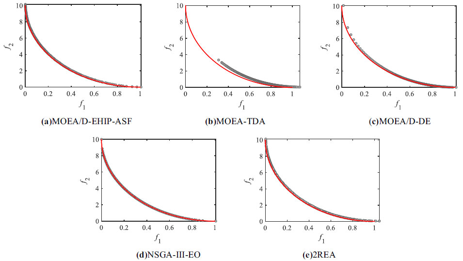 |
Fig. (6). Non-dominated solutions of five evolutionary algorithms for an F1 test problem. |
As can be seen from the table, for the IGD performance metric, MOEA/D-EHIP-ASF outperformed the other compared algorithms due to the use of EHIP, which produced better offspring solutions and promoted the convergence of the algorithm. Moreover, the ideal point-based TCH decomposition strategy and the nadir point-based ASF decomposition strategy are used in the algorithm, which improves the diversity and distribution of the algorithm. Although the diversity and distribution of the algorithm are guaranteed in MOEA/D-MR due to the two reference points, the diversity of the algorithm is further improved with the addition of the ASF decomposition strategy based on the nadir point, indicating that the ASF decomposition strategy based on the nadir point can improve the diversity of the algorithm. For the comprehensive performance metric HV, NSGA-III-EO is better for the multi-optimization problems with linear unimodal PS such as F1, F2, and F3, while MOEA/D-EHIP-ASF is the second best, which is due to the fact that NSGA-III-EO eliminates the worse individuals in the process of selecting solutions instead of selecting the better individuals thus ensuring convergence, which makes the comprehensive performance of the algorithm improve. However, NSGA-III-EO only works well for the PS linear unimodal multi-optimization problem but is less effective for other complicated F-series test problems. The robustness of the proposed algorithm is also improved, as shown by the standard deviations, which makes the algorithm more stable.
In summary, the EHIP can produce better offspring solutions in the evolutionary process and largely improve the convergence of the algorithm two reference points decomposition strategy can well solve the complicated MOPs with extremely convex and extremely concave Pareto fronts, and the ASF decomposition strategy based on the nadir point can further improve the diversity of the algorithm.
 |
Fig. (7). Non-dominated solutions of five evolutionary algorithms for an F2 test problem. |
 |
Fig. (8). Non-dominated solutions of five evolutionary algorithms for an F3 test problem. |
 |
Fig. (9). Non-dominated solutions of five evolutionary algorithms for an F4 test problem. |
 |
Fig. (10). Non-dominated solutions of five evolutionary algorithms for an F5 test problem. |
 |
Fig. (11). Non-dominated solutions of five evolutionary algorithms for an F6 test problem. |
 |
Fig. (12). Non-dominated solutions of five evolutionary algorithms for an F7 test problem. |
 |
Fig. (13). Non-dominated solutions of five evolutionary algorithms for an F8 test problem. |
 |
Fig. (14). Non-dominated solutions of five evolutionary algorithms for an F9 test problem. |
| Test Problems | MOEA/D-EHIP-ASF | MOEA-TDA | MOEA/D-DE | NSGA-III-EO | 2REA |
|---|---|---|---|---|---|
| F1 | 1.926E-2(7.86E-4) | 1.693E+0(2.02E-2) | 1.461E-1(1.60E-2) | 3.823E-2(1.82E-3) | 1.005E-1 (5.22E-2) |
| F2 | 3.326E-3(1.90E-4) | 2.884E-1(1.74E-2) | 9.806E-3(4.03E-4) | 1.126E-2(1.50E-3) | 4.559E-3 (2.04E-4) |
| F3 | 3.909E-3(3.58E-4) | 8.109E-2(1.45E-2) | 9.072E-3(1.72E-3) | 8.071E-3(1.11E-3) | 7.611E-3 (1.33E-3) |
| F4 | 8.809E-3(5.94E-3) | 1.523E-1(5.06E-2) | 6.016E-2(7.24E-3) | 6.236E-2(1.54E-2) | 6.409E-2 (1.77E-2) |
| F5 | 8.054E-3(3.53E-3) | 1.071E-1(2.34E-2) | 3.292E-2(6.24E-3) | 3.883E-2(6.23E-3) | 3.095E-2 (3.58E-3) |
| F6 | 4.542E-3(1.33E-3) | 2.138E-1(1.08E-1) | 3.515E-2(4.90E-2) | 1.001E-1(2.26E-2) | 1.202E-1 (2.49E-2) |
| F7 | 4.758E-3(2.20E-3) | 3.180E-1(9.61E-2) | 1.622E-1(7.78E-2) | 2.056E-1(6.07E-2) | 2.294E-1 (7.12E-2) |
| F8 | 2.700E-2(1.25E-3) | 2.513E-1(1.21E-1) | 5.821E-2(1.53E-2) | 8.641E-2(4.35E-3) | 9.006E-2 (3.55E-2) |
| F9 | 3.973E-2(3.51E-3) | 4.168E-1(1.18E-1) | 1.644E-1(4.34E-2) | 1.367E-1(1.96E-2) | 1.253E-1 (1.14E-2) |
| Test Problems | MOEA/D-EHIP-ASF | MOEA-TDA | MOEA/D-DE | NSGA-III-EO | 2REA |
|---|---|---|---|---|---|
| F1 | 9.841E+0(8.46E-3) | 7.654E+0(1.30E-1) | 9.687E+0(3.07E-2) | 9.915E+0(3.57E-3) | 7.842E-1 (3.49E-3) |
| F2 | 1.156E+0(5.29E-4) | 9.374E-1(4.49E-2) | 1.155E+0(4.16E-4) | 1.158E+0(3.10E-4) | 9.578E-1 (5.47E-5) |
| F3 | 7.037E-1(3.30E-4) | 5.594E-1(2.94E-2) | 7.017E-1(8.60E-4) | 7.068E-1(3.23E-4) | 5.845E-1 (1.42E-4) |
| F4 | 8.546E-1(1.76E-2) | 6.254E-1(5.89E-2) | 7.515E-1(6.39E-3) | 7.388E-1(2.71E-2) | 6.131E-1 (2.68E-2) |
| F5 | 8.536E-1(1.12E-2) | 6.983E-1(2.63E-2) | 7.933E-1(8.91E-3) | 7.855E-1(1.63E-2) | 6.588E-1 (9.87E-3) |
| F6 | 8.678E-1(2.99E-3) | 5.974E-1(6.89E-2) | 7.993E-1(1.01E-1) | 7.100E-1(2.98E-2) | 5.897E-1 (2.14E-2) |
| F7 | 8.677E-1(4.47E-3) | 4.585E-1(9.74E-2) | 5.851E-1(1.22E-1) | 5.662E-1(6.45E-2) | 4.708E-1 (2.92E-2) |
| F8 | 3.066E-1(9.08E-4) | 1.364E-1(5.53E-2) | 2.596E-1(1.78E-2) | 2.201E-1(4.18E-3) | 1.712E-1 (2.74E-2) |
| F9 | 7.343E-1(1.65E-3) | 3.719E-1(9.04E-2) | 6.145E-1(4.71E-2) | 6.132E-1(1.42E-2) | 4.694E-1 (1.04E-2) |
CONCLUSION
In this paper, in response to the poor quality of the offspring solutions generated by the traditional evolutionary operators and the inability of the evolutionary algorithm based on decomposition to better solve the multi-objective optimization problems with complicated Pareto fronts, this paper proposes a multi-objective evolutionary algorithm based on two reference points decomposition and historical information prediction. The EHIP combines linear regression prediction model and differential evolution to generate better quality offspring solutions based on contemporary and historical solutions, which improves the convergence of the algorithm. The TCH based on ideal point and the ASF based on nadir point decomposition strategies solve the multi-objective optimization problem with complicated Pareto front by improving the distribution and diversity. From the experimental results, it can be concluded that the EHIP can generate better quality offspring solutions, and the decomposition strategy based on two reference points can solve the multi-objective optimization problems with complicated Pareto fronts well.
CONSENT FOR PUBLICATION
Not applicable.
AVAILABILITY OF DATA AND MATERIALS
The authors confirm that the data supporting the results and findings of this study are available within the article.
FUNDING
This work is partially supported by the National Natural Science Foundation of China (62063019, 61763026) and the Natural Science Foundation of Gansu Province (20JR10RA152).
CONFLICT OF INTEREST
The authors declare no conflict of interest, financial or otherwise.
ACKNOWLEDGEMENTS
The authors are very grateful to Yang Zhou for his advice on the writing of this article.